Jun 14, 2001 - of the earth's restless oceans and atmoshere, or the gaseous disk of a spiral galaxy. Anything goes, as long as it flows; moreover, the concept of ...
(c)2001 American Institute of Aeronautics & Astronautics or Published with
Permission of Author(s) and/or Author(s)1 Sponsoring Organization.
15th AIAA Computational Fluid Dynamics Conference 11-14 June 2001 Anaheim, CA
AIAA-2001-2520
A01-31039
Computational Fluid Dynamics: Science or Toolbox? Bram van Leer*^ Department of Aerospace Engineering University of Michigan, Ann Arbor, MI 48109-2140 bram@engin. umich. edu
Abstract Over the past six decades the science of CFD has created a versatile computational toolbox. Still, enough barriers remain; for aeronautical CFD one of the highest ones is slow convergence to steady flow solutions. The importance of reducing method complexity to O(N) is discussed in the light of future massively parallel computing. In the same light a vision is outlined of CFD based on PDEs of the lowest possible order, i.e., the first order. Such a methodology will allow significant functional decomposition in addition to domain decomposition. To reap this benefit, a parallel architecture of distributed, sizable clusters of memory-sharing processors is recommended. Removal of computational barriers, and radical innovation will require increased fundamental research on algorithms, implying increased funding for such activity, and continued teaching of method development.
1
Introduction
In its short existence the science of CFD has created a computational toolbox with which many a flowsimulation job can be successfully completed. In fact, the success of CFD methods when applied to certain classes of flow problems is so complete, that users with a limited scope may get the impression all necessary tools are available. Refinement of calculations seems merely a matter of waiting for yet more powerful computers. This view may explain why in the mid-1990s *AIAA Fellow. tCopyright © 2001 by American Institute of Aeronautics and Astronautics, Inc. All rights reserved.
prominent research leaders and program managers could be heard articulating that "CFD is dead." Implied was that CFD as a living science, an area of research and development, was finished, just as the search for the general solution of the quadratic equation is over. What remained was the toolbox, the equivalent of the a&c-formula. I am afraid, though, that behind this statement was something less innocent than mere ignorance: it was used as an excuse to steer funding for computational science away from basic research and in the direction of High-Performance Computing and Communication (HPCC). There is nothing against a wellmotivated policy of moving funding from one research area to another, but it need not be sold to the research community on the basis of a fabrication. We deserve better1. Meanwhile, CFD continues to be a fabulous science full of challenging unsolved problems and opportunities for radical innovation. I hope to convince you of that in what follows. And that toolbox? Well, it just keeps getting fuller.
2
CFD: a mature science
Over the past two decades Computational Fluid Dynamics (CFD) has earned itself a respectable place alongside the established disciplines of theoretical and experimental fluid dynamics. It is a science that attracts numerical analysts, physicists and engineers l l sometimes wonder if we really do. Acceptance of the "CFD is dead" theory was widespread. May one blame someone else for one's own gullibility?
(c)2001 American Institute of Aeronautics & Astronautics or Published with
alike, possibly because of the strong sense of empowerment it confers on its practitioners. The developer of CFD methods creates a virtual reality which users may populate with anything that flows, regardless of scale. It could be a trickle of molecules finding its way through a MEMS microchannel, or the river of air that lifts an entire airplane; it could be the union of the earth's restless oceans and atmoshere, or the gaseous disk of a spiral galaxy. Anything goes, as long as it flows; moreover, the concept of flowing is broad. For example, traffic flows over multilane highways [1] and an ensemble of stars flows through phase space. CFD methods allow us to experiment in our virtual laboratory in ways that would be "expensive, difficult, dangerous or impossible" [2] in the real world. In the six decades of its existence, CFD has removed many barriers - some of them discouragingly high - that stood in the way of successful flow simulation. 1. John von Neumann, who may be called the father of CFD, contributed two major techniques: a practical Fourier method of analyzing finitedifference schemes regarding their stabilty, and the method of artificial viscosity, enabling the capturing of shocks that are likely to arise sooner or later in compressible flow [3].
2. The latter method was significally improved in the early 1970s [4, 5], when it was discovered how non-oscillatory shock profiles could be embedded in smooth flow solutions of high accuracy. 3. Operator splitting [6] gave easy access to multidimensional simulations and the inclusion of extra physical processes. 4. Grid generation, crucial to aerospace and mechanical engineering, came a long way from repeated conformal mapping [7] to the fully automated almost-Cartesian approach [8, 9] with geometry- and flow-adapted refinement, yielding practical grids around complex objects in less than an hour [10]. 5. Searching for steady flow solutions has been greatly facilitated by multigrid [11, 12] and preconditioning [13, 14] techniques.
Permission of Author(s) and/or Author(s)1 Sponsoring Organization.
6. Multi-fluid dynamics has been made accessible to anyone by the powerful level-set method [15], in which the fluid interface is treated as a level surface of an auxiliary distance function.
7. Grid optimization for the accurate computation of key functionals such as lift and drag has become straightforward with the use of the adjoint operator [16]. These are examples; the list is not in any sense complete. Still, enough barriers remain.
3
Some barriers
With the maturing of CFD, our taste for flow problems has matured. Geometric complexity, physical complexity and sheer size are now the three key issues by which CFD methodology is challenged. The modeling of flows in the presence of complex geometry appears to be in good shape, and I believe it will continue to develop for some time without major hurdles to be taken. This is not at all true for the other issues. With regard to the issue of size, the computational cost of computing a steady compressible flow solution with N unknowns generally is far removed from the ideal O(N) operation count. One session of this conference is dedicated solely to that topic: CFD-9, "Multigrid Methods," put together by Jim Thomas (LaRC). It must be emphasized here that massively parallel computing will not bring us any closer to the above theoretical limit. I will address this complex matter in a separate section (Section 4). A challenge in the area of physics is that of turbulence modeling. For most flow configurations there are no reliable turbulence models, and the turbulence models that are in use do not always have desirable numerical properties. While it certainly falls under the mandate of CFD to mold a turbulence model into a numerically robust process, it is not at all clear whether CFD should be given the sole responsibility for turbulence modeling. In this lecture the subject will further be ignored. Related, but fortunately not as hard, is the task of efficiently representing vorticity in compressible flow.
(c)2001 American Institute of Aeronautics & Astronautics or Published with
This will be the subject of Phil Roe's talk [17] later in the session. The last example I want to mention is the challenge of stiff source terms, such as arise in chemically reacting or otherwise relaxing flows. It is trivial to formulate methods that work in the "frozen" limit, in which even the smallest time scale is adequately resolved. But developing methods that do not resolve all scales, yet produce the proper "equilibrium" limit, and, moreover, approach this limit along the proper path [18], is a task we have begun to tackle only in the last few years. Yet, such methods bear the promise of a total make-over of CFD in the 21st century. I will share this vision with you in Section 5.
4
O(N) complexity and parallel computing
Slow convergence to steady compressible-flow solutions is the main reason for stagnation in the design cycle in a discipline like aerospace engineering, where the emphasis is on flow under steady cruising conditions2. There are two independent strategies for reducing turn-around time:
1. divide the computational job over more and more processors; 2. develop more efficient marching algorithms.
The first strategy currently enjoys great popularity among funding agencies and researchers alike, because it is straightforward, viz. it carries low risk. For this strategy to be effective, the computational job must allow distribution over many processors with limited need for interprocessor communication. This requirement favors explicit schemes based on the most compact stencils, as their extreme locality guarantees minimal communication. 2 The same convergence problem arises in unsteady-flow calculations, if the physical processes modelled have strongly disparate time scales, and only the largest scales have to be accurately represented.
Permission of Author(s) and/or Author(s)1 Sponsoring Organization.
Today's most successful CFD codes base the distribution over parallel processors on domain decomposition. Thus, the operation count will scale well if the number of computational cells is several orders of magnitude larger than the number of processors used. For instance, a vista of applying 106 processors to a current-size, « 107-cell science/engineering simulation, is unrealistic, as this is clearly beyond the saturation point of the scaling law. For efficient application of such large numbers of processors to currentsize jobs, additional ways of decomposing must be developed; I shall refer to these as functional decomposition. In particular, we may attempt to assign different PDEs or groups of PDE's to different processors; this would yield the greater benefits for the largest systems. For instance, a system describing chemically reacting flow may exceed 100 equations because of the large number of species to be advected. Therefore, functional decomposition may buy us one or two orders of speed-up. I will revisit this subject in Section 5.3. The second strategy is largely neglected these days, but is crucial to success if one wants to go beyond current-size problems.. This strategy has as its ultimate goal the realization of optimal marching methods, which yield a solution with N unknowns in O(N) operations. This property implies scalability with regard to number of unknowns, and works independently of scalability with regard to number of processors. Convergence in O(N) operations has long been realized for the solution of elliptic equations, owing to the technique of multigrid relaxation [19]. However, for steady solutions to the Euler equations, which include hyperbolic (advective) components, only recently some successes have been reported, e. g., by Darmofal and Siu [20]. In order to make multigrid relaxation yield optimal convergence to Euler and NS solutions, some form of directionality needs to be introduced into the process, to account for the flow direction. How to do this efficiently is still a subject of research. Moreover, implementing multigrid relaxation on parallel processors is not trivial either, because of a difficulty with load balancing. Last but not least, the technique of local preconditioning, needed to equalize advective
(c)2001 American Institute of Aeronautics & Astronautics or Published with
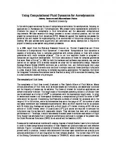
and dissipative time scales before applying multigrid relaxation, is not sufficiently understood and developed for the NS equations [21].. To capture directional effects, Darmofal and Siu use semi-coarsening in two dimensions, after Mulder [22]. This technique is certainly effective, but considered "over-kill": in 3-D it would increase the work by a factor 7 over full coarsening. This does not detract from their most significant result: switching back to full coarsening increases the complexity of the method from O(N) to O(N)%] see Figure 1. For steady Navier-Stokes (NS) solutions the operation count is rather O(7V 2 ) or even worse. Such method complexity ruthlessly disables massively parallel computers: a factor 1,000 increase in the number of processors will allow only a factor y^OOO « 32 more computational cells. Such detail could be obtained in the same wall-clock time by an optimal method with only a 32-fold increase in the number of processors, indicating that the sub-optimal method wastes 96.8% of the processors, e.g., 968,000 out of 1,000,000 processors. Hardware manufacurers may not mind; users, again, deserve better. It is instructive to linger a while with this example. Assume that we are currently satisfied with the resolution and turn-around time of a 3-D NS computation when carried out on a 1000-processor supercomputer. Will PetaFLOPs computing on 106 parallel processors buy us an order of magnitude of grid-refinement in each dimension? If the complexity of the NS methods remains O(JV 2 ), the answer is negative: we will have to wait for ExaFLOPs computing on 109 parallel processors. Now suppose an O(N) method does become available. That immediately makes our current computers more powerful. Assuming the O(N2) method was competitive with the O(N) method for problems fitting on a single workstation, it follows we may now obtain on a 32-processor workstation those 3-D NS solutions that used to require the power of 1000 processors. Resolution improvement of an order of magnitude in each dimension will be feasible in constant wall-clock time on just 32,000 processors. That kind of hardware may appear relatively soon. Throughout this example I have assumed, for simplicity, that the computations scale perfectly with the
Permission of Author(s) and/or Author(s)1 Sponsoring Organization.
number of processors. That sort of scalability is in a pretty good shape, which has been achieved even on self-adaptive grids Just wait for Ken Powell's talk [23] in this session, describing almost perfect scalability up to 1490 processors for MHD computations on blockwise self-adapting grids. My point is that we equally need scalability with regard to number of unknowns, and we haven't got it yet.
5 5.1
A Vision Scalable PDE's
CFD
by
First-Order
Computational Fluid Dynamics (CFD) may be due for a new generation of algorithms that will extract the maximum benefit from future massively parallel computer architectures. Even though today's CFD techniques already are quite well geared for parallel processing (cf. Powell's contribution [23]), I believe that there is still much to be gained by rethinking CFD algorithms. It is my view of the future that the most efficient, most generally useful numerical methods for flow simulation will continue to be based on a description of the flow physics by PDE's, discretized on a computational grid. At present I see no reason to abandon such methods in favor of more exotic simulation methods. Cellular automata, lattice-Boltzmann methods and other discrete-particle methods all have special-purpose uses, but their intrinsic low accuracy and statistical noise make them unsuited for general problem-solving in fluid dynamics; see, e. g., Lockard et al. [24]. What distinguishes my vision and that of my collaborators is that we believe the flow physics should be expressed in PDE's of the lowest possible order, that is, the first order. Such PDEs only contain advection terms and local, possibly stiff source terms; these are called hyperbolic-relaxation equations. The source terms are responsible for attenuation, traditionally the role of second-order and higher-evenorder dissipation terms. How to develop such a description is not trivial and will be addressed further below.
Permission of Author(s) and/or Author(s)1 Sponsoring Organization.
(c)2001 American Institute of Aeronautics & Astronautics or Published with
10000 9000 8000 7000 6000
5 I 5000
* 4000 3000 2000 1000
2
2.5 : Number of cells
4.5
5 x 10⁴
Figure 1: CPU seconds versus number of cells, N. NACA 0012 flow with preconditioned Jacobi at M^ = 0.1. x : full-coarsening; o: semi-coarsening. Curve fits are given by CPUfuu = (8.2 x 10~4)JVi and CPUsemi — (3.8 x W~2)N. From Darmofal and Siu [20]. A first-order system generated this way is always larger than the equivalent traditional system of conservation laws; for instance, a well-posed hyperbolic first-order system equivalent to the 3-D Navier-Stokes (NS) equations includes separate evolutionary equations for the 6 different elements of the pressure tensor and the 3 heat fluxes. This seeming computational disadvantage is only superficial: much of the additional updating amounts to evaluating NS terms under a different name, yielding comparable update timings [25]. Moreover, any overhead is handsomely compensated for by a host of computational advantages of the first-order formulation, especially in a future of massively parallel computing on non-smooth grids.
1. First-order PDE's require the smallest possible stencil for accurate discretization, therefore the least need for internodal communication. This is an obvious advantage in parallel computing. 2. Whereas traditional viscosity and conduction terms cause global stiffness that calls for a globally implicit integration, stiffness of a local source term can be overcome by a local im-
plicit integration, without any need for internodal communication.
3. Discretized first-order systems may be easier to drive to convergence than equivalent higher-order systems, some evidence in this regard can be found in the steady-shock calculations of Brown [25]. 4. First-order PDE's yield the highest potential discretization accuracy on non-smooth, adaptively refined grids. It has been known for some time that second-order dissipation terms can not be discretized on a non-smooth grid without loss of accuracy (or even consistency), compactness and/or positivity [26]; this problem is avoided with the use of first-order PDE's.
5. The larger systems of first-order PDE's are better suited for functional decomposition than the traditional higher-order systems, specifically, for decomposition by equations or groups of equations. This type of decomposition would work in tandem with domain decomposition, allowing the use of more processors on a fixed-size job.
(c)2001 American Institute of Aeronautics & Astronautics or Published with
Thus, the increased system size may even lead to reduced wall-clock time. Necessary for such decomposition to work is a multilevel parallel architecture, i. e., distributed, sizable clusters of memory-sharing processors. 6. First-order PDE's can be used to describe extended hydrodynamics, i. e., flow at intermediate Knudsen numbers [27], encountered in miniature MEMS devices as well as around spacecraft. Traditional descriptions based on higher-order PDE's (Burnett and Super-Burnett equations) require larger stencils, reducing accuracy on nonsmooth grids and parallelizability, while DirectSimulation Monte-Carlo (DSMC) methods are suited only for high-speed flow.
Permission of Author(s) and/or Author(s)1 Sponsoring Organization.
Accurate numerical integration of the hyperbolic system (2) can be accomplished with an explicit highresolution scheme, provided the time step used is sufficiently shorter than the relaxation time scale r. However, if one is interested only in the longer time scales, use of large time steps would be desirable. To keep the integration stable, an obvious but naive approach would be to treat the stiff source term implicitly. However, as indicated already by Arora [28] this does not necessarily yield an accurate equilibrium solution, i. e., one satisfying Eq. (4). To achieve such accuracy, source term and fluxes must be strongly coupled; using fluxes based on the frozen physics is not adequate. One way to establish the coupling between source and fluxes is through a change of state variables that removes the source term. The transformation
For the sake of completeness, below are presented some technical details about hyperbolic-relaxation q = e rr systems and their numerical approximation (Section 5.2), followed by a discussion of the use and imple- reduces the system (2) to mentation of functional decomposition (Section 5.3). r*
5.2
-
(5)
0,
r, - o;
Hyperbolic-relaxation equations
(6) (7)
A model for hyperbolizing a diffusion equation is the the source term has disappeared but the relaxation two-equation system called the hyperbolic heat equa- time now shows up as a weighting factor in state vari-
tion:
ables and fluxes. Numerical fluxes based on this formulation have the potential of achieving solution ac= 0, (1) curacy in both asymptotic regimes, and in between. K qq A model closer to fluid dynamics is the more gen-; (2) eral linear system analyzed by Hittinger [18]: here T and q represent temperature and heat flux, K is + vx = 0, (8) the conductivity, and r is the relaxation time. When — V r is very small, the PDE for the heat flux reduces to CL U = (9) the classical relation where ap is the signal speed according to the frozen q = -KTX (3) physics, and &E is the equilibrium signal speed. Igwhich reduces the evolution equation for the temper- noring the source term, we find the characteristic speeds of the system are ±a/r; the second equation, ature to the standard diffusion equation though, tends to the equilibrium relation F
Tt = KT~.
X
(4)
v=
(10)
Solutions of this system show undamped waves moving at speeds ±-^/(/c/r) for times short compared to which makes the first equation tend to the advection T (the "frozen" limit), and a diffuse distribution for equation large times (the "equilibrium" limit) . ut + (IEUX = 0, (11)
(c)2001 American Institute of Aeronautics & Astronautics or Published with
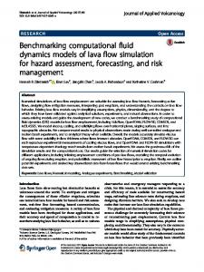
with advection speed CLE- Hittinger presents exact solutions to Riemann initial-value problems for (9); an example is given in Figure 2. He also analyzes the solution to the Riemann problem for the general linear hyperbolic-relaxation system + Ails = Qu,
(12)
where A is an m x m matrix with a complete set of real eigenvectors, and Q is of rank n < m, with nonpositive eigenvalues. This leads to ra — n equilibrium equations. Since a closed-form exact solution can not be given, Hittinger derives leading terms of the asymtotic equilibrium solution. He shows that an approximate equilibrium solution can be combined with the frozen Riemann solution for the development of a numerical flux function valid in all regimes. This is illustrated with numerical solutions to discontinuous initial-value problems. All systems discussed so far are linear; fluiddynamical conservation laws, though, are nonlinear. This complicates the application of the transformation (5), which is now ruled by the solutiondependent matrix exp[—Q(u)t/r]. Averaging and local linearization are required at each time level, making the calculation of numerical fluxes costly. Hittinger indicates that flux functions of the HartenLax-Van Leer (HLL) [29] type, which use only very limited information about the exact solution, may be the most practical way to go for nonlinear gasdynamics. Linde [30] recently presented an highly promising HLL-type flux formula that recognizes single discontinuities (just as Roe's [31]) at a cost per equation independent of the system size. At present, developing an asymptotically correct HLL flux is the key research issue in the hyperbolic-relaxation approach to CFD. Another important issue, though less pressing, is how to make high-resolution schemes for these systems monotonicity preserving over the entire range of the relaxation parameter. It is comparatively easy to achieve this for schemes intended solely for marching to steady solutions; for this purpose the use of locally steady subcell distributions [32] has proved successful. However, for general acceptance of the hyperbolicrelaxation approach we must insist on equally good performance when computing transient flows.
Permission of Author(s) and/or Author(s)1 Sponsoring Organization.
Hyperbolic-relaxation systems for gas dynamics and their numerical implementation have been studied intensively at the University of Michigan, by Arora, Brown [25, 33], Groth [27] and Hittinger. The best-known system to date is that of the 10-moment equations; it describes viscous nonconducting flow. The equations are obtained by taking 10 different moments of the Boltzmann equation, using a generalized Gaussian distribution function (following Levermore [34]), and evaluating the collision integrals in the BGK approximation. The usual energy equation is replaced by 6 equations for the different elements of the pressure tensor. Hittinger has extended the equations to include relaxation of both translational and rotational degrees of freedom, for the description of gases like air. Brown used an explicit high-resolution scheme to compute steady shock profiles for the 10-moment equations. He showed this requires less CPU time (from a factor 1/2 at Mach 1.1 down to 1/16 for Mach 10) than for the NS equations. Groth [27] computed shock structures for a rarefied gas at intermediate Knudsen numbers, and showed that these match the structures computed at much greater expense with a DSMC method. For a well-posed description of 3-D viscous conducting flow at least 14 equations are needed. Up to 35 equations [25] have been used in describing larger deviations from thermodynamic equilibrium3. These are sizable systems, pre-eminently suited for functional decomposition of the kind described in the next subsection.
5.3
Domain and functional decomposition for parallel computing
For distributed-memory MIMD architectures, domain decomposition and message passing have proved to be very effective means of achieving parallelism in CFD computations on thousands of processors (cf. Powell's contribution [23] to this session). As mentioned in Section 3, though, this approach will reach the limit of saturation rather easily on future, mas3
Brown has also calculated steady-shock profiles for the 35moment system.
(c)2001 American Institute of Aeronautics & Astronautics or Published with
Permission of Author(s) and/or Author(s)1 Sponsoring Organization.
200
20
u/uf
U/Uf
15
150
10
.100
50
-10
-5
0
10
0 -100
-50
0
50
100
0
50
100
x/aFT
200
z/aFuc 150
JOO
50
-100
-50
x/a,
Figure 2: Resolution of a discontinuity according to the first-order system (9); plotted are contours of u (top) and z = v — CLEU (bottom) in the x — t plane. Left: details of wave propagation in the solution for short times. Right: the solution viewed on a larger time-scale resembles an advection-diffusion solution for u, while z uniformly tends to zero. From Hittinger [18].
(c)2001 American Institute of Aeronautics & Astronautics or Published with
Permission of Author(s) and/or Author(s)1 Sponsoring Organization.
tioned into 10,000 groups, each group containing 100 processors. Each processor group will be assigned to a different zone with 1000 cells. It is essential now that each processor in a group keeps all data computed for the zone by the entire group, so that data communication (if any) is minimal; this will allow functional decomposition within each group of processors. Thus, the 100 processors in each group must have shared memory, while the inter-group memory may be distributed. Such an architecture is ideal for parallelizing a CFD code based on first-order PDE's.
sively parallel machines. This means we have to explore other roads to parallelism. As to shared-memory machines, currently one can readily buy boards with 2 and 4 processors sharing memory; however, there appears to be a major technical barrier when trying to push shared-memory architecture beyond 32 processors. Besides shared-memory and distributed-memory architectures there are multilevel-memory architectures, in which some processors have both private and shared memories. We believe future massively parallel computers, with w 1 million processors, will fall into this category. In the detailed example given further below we assume the availability of 100-processor shared-memory clusters4, in order to illustrate all different levels of parallelism allowed by our approach to CFD. We shall map a 10-million-cell problem (typical for, e. g., a full-aircraft design) onto 1 million processors. The following strategy fully utilize the processors in pursuit of minimizing turn-around time.
Step 2. Functional decomposition. The most obvious functional decomposition is to let each of the 100 processors in a group solve a different PDE of the first-order PDE system. Thus, the more equations there are in the system, the greater the potential for this type of parallelism. The five 3-D NS equations can be rewritten as a first-order system of fourteen equations, a considerable gain in size, but still a factor « 7 short of providing a task for each processor. In this case one could simply assign seven zones to each group5. Another solution lies in outer-loop parallelization,not further discussed here. If, however, we consider flow with chemical reactions, we may easily have a hundred or more equations governing the evolution of all species. In this case, the 100 processors in each group will have plenty to work on just by functional decomposition. No data exchange is necessary at any time between the processors in the group because they share the same memory and data.
Step 1. Domain and processor decomposition. The domain is partitioned into about 10,000 zones with the cells equally distributed over the zones, i.e., about 1,000 cells per zone. This is large enough a size to have a good preponderance of interior cells, where the work is done, over ghost cells (copies of cells from neighboring zones) needed for updates near the zone boundaties. (For example, the MHD code [35] that performed the calculation of Coronal Mass Ejection (CME) to be presented by Powell, assigns one or more blocks of 1000 cells to each processor.) Care must be taken to minimize the number of interfaces, so as to reduce communication overhead. A variety of algorithms such as the Recursive Spectral Bisection algorithm [36] can be used for domain partitioning. Alternatively, as in Powell's CME calculation, the zones may be automatically generated as a result of adaptive grid refinement.
Meanwhile, the 1 million processors are parti4 Note that a network of 14-processor shared-memory workstations would already allow full functional decomposition for simulations of viscous conducting flow using first-order PDE's.
In order to achieve the best performance, the functional decomposition must be fine-tuned for optimal load balance. For example, depending on the computational intensity of each equation, we may assign several equations to one processor or solve one equation on several processors. If it becomes necessary to split the load of solving 5
The alternative, further decomposition of one zone into 7 subzones, is not practical because the ratio of ghost cells to interior cells per subzone gets too large. Even with shared memory this will cause loss of efficiency due to excessive data migration.
Permission of Author(s) and/or Author(s)1 Sponsoring Organization.
(c)2001 American Institute of Aeronautics & Astronautics or Published with
one equation over several processors, outer-loop in turn influence IT research, as the new methodparallelization is a further possibility. Details are ology offers the broadest possible proving ground omitted here. (within the bounds of PDE-solving) for massively parallel computing. I even submit that the apparent In summary, with domain decomposition and funcsymbiosis between the first-order description and tional decomposition (and, possibly, outer-loop parmultilevel parallel architectures may contribute allelization) we are confident to be able to achieve to the evolution of scientific computers toward a near-optimum efficiency on tomorrow's parallel maparallel architecture of distributed, sizable clusters chines. Using the largest possible PDE systems inof memory-sharing processors. stead of the traditional smaller sets of flow equations will be a significant advantage. Now, back to reality. The funding emphasis on HPCC applications, rather than on basic research, persists to this day6. It is unlikely that this situa6 Conclusions and outlook tion will change as long as most users of CFD tools In this lecture I have attempted to show by example have yet to encounter the practical limit to massively that CFD as a science is alive and well. parallel computing. Until that day, advances in CFD will be expected I have indicated one big hurdle, the high complex- to come mainly from advances in hardware. I hope ity of steady-flow methods. Its removal will require that by that time there will still be some individuals all of our ingenuity, and considerably greater man- left with the knowledge to develop a new generation power, i. e., increased funding for basic research. of CFD methods. Better yet, let us prepare for that If massively parallel computing is realized without day by continuing to educate CFD students in the a significant reduction in method complexity, the area of method development. power of most processors, hundreds of thousands of them, will be wasted. In contrast, if a reduction in complexity is achieved soon, we won't have to wait for the arrival of PetaFLOPs computing in order to Acknowledgements achieve a quantum jump improvement in resolution. I am indebted to my colleagues Phil Roe, Ken Powell I have also sketched an opportunity for a radical in- (University of Michigan) and Z. J. Wang (Michigan novation of CFD, with particular regard to a future of State University), and to Jeff Hittinger (Lawrence massively parallel computing on adaptive grids. It is Livermore National Laboratory), for their contribua vision of CFD based on large systems of first-order tions to developing the vision of "Scalable CFD by hyperbolic-relaxation PDEs. Such systems combine First-Order PDEs", first expressed in a research prowell with functional decomposition, needed to sup- posal to NASA. I am particularly grateful to Z. J. for plement domain decomposition when distributing a sharing his ideas on functional decomposition and the computational job over many processors. Realizing future of parallel architecture. Most of the text of this vision will require substantial fundamental re- Section 5.3 is his. I also thank David Darmofal and search in both numerical analysis and computer sci- Jeff Hittinger for allowing the use of Figures 1 and 2, ence. respectively. A general shift toward the above CFD method6 ology will not only transform CFD but also have a The last months of the Clinton-Gore government, though, have brought some announcements by major funding agencies profound impact on research and learning in fluid (NSF, DOE, even NASA) inviting proposals for fundamental dynamics, since it calls for adopting a non-traditional research on algorithms. It is not at all clear if these herald a fluid description. While the motivation for this shift shift in emphasis at the agencies, and, if indeed so, whether or is rooted in part in information technology, it will not this trend will survive the change of government.
10
(c)2001 American Institute of Aeronautics & Astronautics or Published with
References [I] S. P. Hoogendoorn, Multiclass Continuum Modeling ofMultilane Traffic Flow. PhD thesis, Delft University of Technology, 1998. [2] P. L. Roe, "Introduction to computational fluid dynamics." Lecture Notes to a Short Course at Cranfield Institute of Technology, May 27-29,, 1986.
[3] R. D. Richtmyer and K. W. Morton, Difference Methods for Initial-Value Problems. Interscience, 1967.
Permission of Author(s) and/or Author(s)1 Sponsoring Organization.
[13] B. van Leer, W. T. Lee, and P. L. Roe, "Characteristic time-stepping or local preconditioning of the Euler equations," AIAA Paper 91-1552-CP, 1991. [14] D. L. Darmofal and K. Siu, "A robust locally preconditioned multigrid algorithm for the Euler equations," AIAA Paper 98-2428, 1998. [15] W. Mulder, S. Osher, and J. A. Sethian, "Computing interface motion in compressible gas dynamics," Journal of Computational Physics, vol. 100, pp. 209-228, 1992.
[4] J. P. Boris and D. L. Book, "Flux-Corrected [16] D. A. Venditti and D. L. Darmofal, "AdTransport I: SHASTA, a fluid-transport algojoint error estimation and grid adaptation for rithm that works," Journal of Computational functional outputs: Application to quasi-onePhysics, vol. 11, pp. 38-69, 1973. dimensional flow," Journal of Computational Physics, vol. 164, pp. 204-227, 2000. [5] B. van Leer, "Towards the ultimate conservative
[6] [7]
[8]
[9]
[10]
[II] [12]
difference scheme. I. The quest of monoticity," [17] P. L. Roe, "Capturing vorticity," in AIAA Lecture Notes in Physics, vol. 18, pp. 163-168, 15th Computational Fluid Dynamics Confer1973. ence, AIAA 2001-2523-CP, 2001. N. N. Yanenko, The Method of Fractional Steps. [18] J. A. Hittinger, Foundations for the GeneralizaSpringer, 1971. tion of the Godunov Method to Hyperbolic SysG. Moretti, "Efficient Euler solver with many tems with Stiff Relaxation Source Terms. PhD applications," AIAA Journal, vol. 26, pp. 655thesis, University of Michigan, 2000. 660, 1988. M. J. Aftosmis, J. Melton, and M. Berger, [19] A. Brandt, "Guide to multigrid development," in Multigrid Methods (W. Hackbush and U. Trot"Adaptation and surface modeling for Cartesian tenberg, eds.), no. 960 in Lecture Notes in Mathmesh methods," AIAA Paper 95-1725-CP, 1995. ematics, Springer Verlag, 1982. S. Bayyuk, A Method for Simulation Flows with Moving Boundaries and Fluid-Structure Interac- [20] D. Darmofal and K. Siu, "A robust multigrid algorithm for the Euler equations with local pretions. PhD thesis, AFOSR, 1999. conditioning and semi-coarsening," Journal of J. C. T. Wang and G. F. Widhopf, "Anisotropic Computational Physics, vol. 151, pp. 728-756, cartesian grid method for viscous turbulent 1999. flow," AIAA Paper 2000-0395, 2000. A. Brandt, "Multilevel adaptive computations in [21] D. Lee, "The design of Navier-Stokes preconditioing for compressible flow," Journal of Comfluid dynamics," AIAA Journal, voL 18, 1980. putational Physics, vol. 144, pp. 460-483, 1998. W. A. Mulder, "A new multigrid approach to convection problems," CAM Report 88-04, [22] W. A. Mulder, "A new approach to convection UCLA Computational and Applied Mathematproblems," Journal of Computational Physics, ics, 1988. vol. 83, pp. 303-323, 1989. 11
Permission of Author(s) and/or Author(s)1 Sponsoring Organization.
(c)2001 American Institute of Aeronautics & Astronautics or Published with
[23] K. Powell, G. Toth, D. DeZeeuw, P. Roe, and [32] B. van Leer, "On the relation between T. Gombosi, "Development and validation of the upwind-differencing schemes of Godunov, Engquist-Osher and Roe," SIAM Journal on solution-adaptive, parallel methods for comScientific and Statistical Computing, vol. 5, pressible plasmas," in AIAA 15th Computational Fluid Dynamics Conference, AIAA 20011984. 2525-CP, 2001. [33] S. L. Brown, P. L. Roe, and C. P. T. Groth, "Numerical solution of 10-moment model [24] D. P. Lockard, L.-S. Luo, and B. A. Singer, for nonequilibrium gasdynamics," AIAA Paper "Evaluation of the Lattice-Boltzmann equaAIAA Paper 95-1677, 1995. tion solver Powerflow for aerodynamics applications." ICASE Report 2000-40, 2000. [34] C. D. Levermore, "Moment closure hierarchies for kinetic theories," J. Stat. Phys., vol. 83, [25] S. L. Brown, Approximate Riemann Solvers for pp. 1021-1065, 1996. Moment Models of dilute Gases. PhD thesis, University of Michigan, 1996. [35] K. G. Powell, P. L. Roe, T. J. Linde, D. L. DeZeeuw, and T. I. Gombosi, "A solution[26] W. J. Coirier and K. G. Powell, "An accuadaptive upwind scheme for ideal magneracy assessment of Cartesian-mesh approaches tohydrodynamics," Journal of Computational for the Euler equations," AIAA Paper 93-3335Physics, vol. 154, pp. 284-309, 1999. CP, 1993. [27] C. P. T. Groth, "Devolpment of godunov meth- [36] A. Pothen, H. Simon, and K. P. Liou, "Partitioning space matrices with eigenvector of graphs," ods for hyperbolic momentum equations of exSIAM J. Mat. Anal Appl, vol. 11, pp. 430-452, tended hydrodynamics," in Godunov's Method 1990. for Gasdynamics: Current Applications and Future Developments (B. van Leer, ed.), University of Michigan, 1997. [28] M. Arora, Explicit Characteristic-Based HighResolution Algorithms For Hyperbolic Conservation Laws with Stiff Source Terms. PhD thesis, University of Michigan, 1996.
[29] A. Harten, P. D. Lax, and B. van Leer, "Upstream differencing and Godunov-type schemes for hyperbolic conservation laws," SI AM Review, vol. 25, pp. 35-61, 1983. [30] T. Linde, "A practical, general-purpose Riemann solver for hyperbolic conservation laws," in Numerical Methods in Fluid Dynamics VII, Seventh International Conference on Numerical Methods for Fluid Dynamics, to appear in 2001. [31] P. L. Roe, "Approximate Riemann solvers, parameter vectors and difference schemes," Journal of Computational Physics, vol. 43, pp. 357372, 1981. 12