Computational Geometry Based Placement Migration - Computer

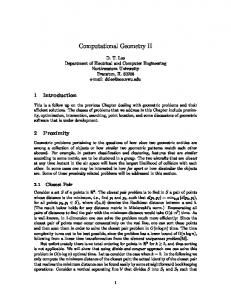
Computational Geometry Based Placement Migration †

Tao Luo† , Haoxing Ren†‡ , Charles J. Alpert‡ , and David Z. Pan† Department of ECE, University of Texas at Austin, Austin TX 78712 ‡ IBM Corporation, 11400 Burnet Road, Austin TX 78758 {tluo, dpan}@ece.utexas.edu, {haoxing, alpert}@us.ibm.com

ABSTRACT Placement migration is a critical step to address a variety of postplacement design closure issues, such as timing, routing congestion, signal integrity, and heat distribution. To fix a design problem, one would like to perturb the design as little as possible while preserving the integrity of the original placement. This work presents a novel computational geometry based placement migration method, and a new stability metric to more accurately measure the “similarity” between two placements. It has two stages, a bin-based spreading at coarse scale and a Delaunay triangulation based spreading at finer grain. It has clear advantage over conventional legalization algorithms such that the neighborhood characteristics of the original placement are preserved. Thus, the placement migration is much more stable, which is important to maintain. Applying this technique to placement legalization demonstrates significant improvements in wire length and stability compared to other popular legalization algorithms.

1.

INTRODUCTION

In modern placement and physical synthesis of VLSI circuits, one is increasingly faced with the placement migration problem, which is to take an existing placement, fix some design violations and re-legalize it. For example, during physical synthesis or Engineering Change Order (ECO) optimization, many buffers may be inserted and gates resized, creating a lot of overlapping cells. These cells need to be legalized, but one should avoid disturbing the previous placement too much to achieve design convergence. Also another example, post routing congestion analysis may identify severe hot spots (e.g., congestion, noise, power, thermal), and placement migration is needed to smoothly spread out cells in these hot spots [1]. Due to the complexity of modern nanometer designs, it is unlikely to design one placement algorithm that meets the multi-objective design closure target in a single run. More often, a placement flow involves multiple placement-improvement iterations. So a stable placement migration algorithm is crucial for the multi-objective design closure. These tasks share a common theme of starting with an initial placement that is “good” and perturbing it so that it is improved in some way while still preserving the essential characteristics (cell ordering, wirelength, etc.) of the original placement. Ideally, the later placement iteration should be able to preserve previous fixes and accumulate additional improvements to achieve the design closure. Therefore, the stability of the placement algorithm is very important. Obviously, we do not want each placement iteration generThis work is supported in part by SRC under contract 2005-TJ1321, IBM Faculty Award, Sun, and equipment donations from Intel.

ates entirely different result and destroys all previous optimization efforts. Among various placement migration applications, legalization is probably the most common one. Therefore, the remainder of the paper will discuss our placement migration algorithm in this context. Existing legalization techniques for legalization include network flow [2] [3], dynamic programming [4][5], heuristic ripple cell movement [6], and single row optimization [7] [8]. The network flow approach [3] uses minimum cost flows to minimize the weighted sum of (squared) cell movements. The dynamic programming based approach [4] solves the optimal assignment of cells to placement sites under the constraint of cell ordering. Mongrel [6] uses a greedy heuristic to move cells from overflowed bins to under capacity bins in a ripple fashion based on total wire length (TWL) gain. The single row optimization techniques [7] [8] use dynamic programming to optimally place cells in a single circuit row. While there are many existing legalization algorithms, there are very few works directly targeting incremental and stable placement migration.1 In this paper, we develop a novel technique for stable placement migration based on the computational geometry. We also propose a new placement stability metric which can be used to measure the placement migration stability. Our algorithm has two key steps: bin-based cell spreading and Delaunay triangulation based overlap reduction. The algorithm takes advantage of the computational geometry property of the existing placement. Thus it captures the relative cell order nicely during placement migration. Our experimental results compared to other widely used legalization algorithms clearly demonstrate the superiority of our algorithm, with over 10% wire length reduction and significantly better stability score. The rest of the paper is organized as follows. Section 2 presents the bin based spreading algorithm. Section 3 presents the Delaunay based overlap reduction procedure. The complete computational geometry based legalization algorithm is given in section 4. Section 5 proposes a new placement stability metric suitable for placement migration. Very promising experimental results are obtained in section 6, followed by conclusion in section 7.

2.

BIN BASED SPREADING

A placement is close to legal if all that is required to legalize the placement is to snap cells to rows or perhaps perform minor cell sliding in order to fit the cells. Assuming the chip layout is divided into equal sized bins, the placement is considered close to 1 The most recent work on diffusion-based placement [7]simulates the placement spreading using the physical diffusion equation. It shares some common theme with this work, but using very different approaches. See Section 6 for more discussion on these two approaches.

legal if the area density of every bin is less than or equal to Dmax (e.g., Dmax = 1). For all bins with density greater than Dmax , cells must be migrated to other bins. Therefore the goal of our migration algorithm is to reduce the density of each bin to no more than Dmax while avoiding moving these cells far from their original locations thus preserving the original placement characteristics. Bin based spreading is a geometric approach to evenly reduce cell density on the congested regions. Suppose we divide the entire placement region into K*L square bins, there will be (K + 1)*(L + 1) bin corners. The idea is to move those bin corners such that the resulting bin capacity would satisfy the density constraints, and then move cells accordingly. By stretching the bin corners, we preserve the relative order of neighboring bins; meanwhile by interpolating cells relative to its bin corners, we preserve the relative order of cells inside the bin. We perform the bin stretching and cell interpolation iteratively until all the bins are under the maximum density Dmax .

2.1

Bin Stretching

At each iteration, we first compute the bin density Dk,l (n) (the nth iteration), then compute the amount of stretching needed for each bin. For those overpopulated bins, the idea is to expand that bin such that the density of the new bin is equal to Dmax . At the same time, to accelerate the spreading process, we allow the adjacent bins to shrink such that their densities equal to Dmax as well. The amount of stretching for bin (k, l) on both horizontal and vertical directions can be written as: s Dk,l (n) x − 1)W εk,l = ( Dmax s Dk,l (n) y εk,l = ( − 1)H (1) Dmax where W and H are the bin width and height, respectively. Stretching each bin itself would generate overlaps between adjacent bins. Therefore we stretch the bin corners of adjacent bins y instead of bins itself. Let (pxk,l (n), pk,l (n)) denotes the coordinates of an inner bin corner, which is shared by four neighboring bins, denoted as (k − 1, l − 1), (k − 1, l),(k, l − 1), and (k, l). We can use (1) to compute the amount of horizontal and vertical stretching needed for each one of the four bins, which will give us four stretched corner positions, and then compute the combined number of these four y as the corner position for next iteration, (pxk,l (n + 1), pk,l (n + 1)), pxk,l (n + 1) = pxk,l (n) + 0.5(εxk−1,l−1 + εxk−1,l − εxk,l−1 − εxk,l ) y

y

y

y

y

y

pk,l (n + 1) = pk,l (n) + 0.5(εk−1,l−1 + εk,l−1 − εk−1,l − εk,l )

B4,4 p4,4 (n)

B3,3

B4,3

B3,4 p4,4 (n+1) B 4,4 B3,3

2.2

B4,3

Figure 1: Illustration of bin and corner stretching Figure 1 is an illustration of the movement of the corner point p4,4 under accumulated stretching from all four surrounding bins. Bin (3, 3), (4, 3), and (4, 4) are over the maximum density, therefore we expand them, while bin (3, 4) is under the maximum density, thus we compact it. We will have four new corner positions of

Cell Interpolation pk,l(n+1) pk,l(n)

pk-1,l(n)

pk-1,l(n+1) x(n+1),y(n+1)

x(n),y(n)

β pk-1,l-1(n)

α

pk,l-1(n) p k-1,l-1(n+1)

α

β pk,l-1(n+1)

Figure 2: Cell location interpolation on stretched bin The computation of new cell coordinates is a linear interpolation process, which maps all cells from the original bin into the new bin at the same relative positions. As shown in Figure 2, the four corner coordinates of the bin are pk−1,l−1 (n), pk,l−1 (n), pk−1,l (n), and pk,l (n) . Their coordinates after bin stretching are: pk−1,l−1 (n + 1), pk,l−1 (n + 1), pk−1,l (n + 1), and pk,l (n + 1). For a cell (x(n), y(n)) within the bin, the new coordinates x(n + 1) and y(n + 1) can be computed by the following equations. x(n + 1) =

γx + β(ξx − γx )

y(n + 1) =

γy + α(ξy − γy )

(3)

where α

=

β

=

γx

=

ξx

=

γy

=

ξy

=

x(n) − pxk−1,l−1 (n) pxk,l−1 (n) − pxk−1,l−1 (n) y y(n) − pk−1,l−1 (n) y y pk−1,l (n) − pk−1,l−1 (n) pxk−1,l−1 (n + 1) + α(pxk,l−1 (n + 1) − pxk−1,l−1 (n + 1)) pxk−1,l (n + 1) + α(pxk,l (n + 1) − pxk−1,l (n + 1)) y y y pk−1,l−1 (n + 1) + β(pk−1,l (n + 1) − pk−1,l−1 (n + 1)) y y y pk,l−1 (n + 1) + β(pk,l (n + 1) − pk,l−1 (n + 1))

(4)

2.3 (2)

Because the stretching is uniform on both bin corners on the same bin edge, we only take half the stretching value given by (1). If any neighboring bin is on the chip boundary, we take the 0.5 factor off. B3,4

this corner for each bin. Such process is iterated as needed. After computing coordinates of all points, cells inside the bin will move within the distorted bin as explained in next section.

Bin Based Spreading Algorithm

At each iteration of the bin based spreading algorithm, it first stretches the bin corner to make congested bin larger, then interpolates cell locations accordingly. It then restores all the bin boundary and starts an new iteration. The new iteration recomputes the bin density and repeats all above procedures. The process stops once that all the bin densities are lower than the maximum density Dmax . To avoid over expansion in non-congested region, we only change the bin corners of those bins above Dmax during bin stretching. It assures that cells are pushed from high density area to low density area steadily and smoothly. It also reduces unnecessary oscillation and computations. The stability of the migration process is affected by the bin size (area) as well. The ideal initial bin size is depending on the size of the circuits. If the bin size is too large, the internal density distribution inside the bin might still violate the density constraints even if the bin as a whole is under Dmax . However, if the bin size is too small, oscillation will appear and bin boundary distortion may impact the smoothness of spreading. We may see cells tend

to cluster in some areas. This problem is solved by a hierarchical addition to our original formulation. The idea is straightforward. It uses big bin sizes from at the beginning, then recursively cuts big bins into smaller bins, and adjusts the internal density distribution. The hierarchical technique is necessary to handle fixed macros. At the time the bin size is smaller enough, bin edges be close to macro boundaries. Cells will move along the boundary, they will not move toward the macros. The complete bin based spreading algorithm is given by Algorithm 1. Algorithm 1 Computational Geometry Bin Based Spreading 1: Procedure: BIN 2: Input: cell placement xi , yi , bin area AB = W · H, maximum bin density Dmax 3: Output: new placement xˆi , yˆi 4: begin Initialize bin density Dk,l ; 5: 6: if AB is too small then return; 7: while any Dk,l > Dmax 8: for each bin with Dk,l > Dmax y 9: Compute bin expansion εxk,l , εk,l with (1); 10: end for 11: Compute bin corner pk,l (n + 1) with (2); 12: Interpolate cell locations xi (n + 1), yi (n + 1) with (3); 13: Restore all bin corners, update Dk,l ; 14: n = n + 1; 15: end while 16: Update xˆi = xi (n), yˆi = yi (n); 17: Reduce bin area AB = AB /2; 18: Recursively call BIN( xˆi , yˆi , AB , Dmax ); 19: end Note that our approach is different from the grid warping [9] and cell shifting [10]. At each partition step, grid warping slices the region into 2 x 2 or 4 x 4 equal “volume” quadrilateral grids, transforming the grid (and cells) back to equal shape rectangles to form the subproblems. The elastic grids in grid warping are the equivalence to Gordian’s min-cut partition [11], both purpose is for partition, while our bins are used for spreading directly. We reshape each bin individually at each step and rely on iterations to flow cells out eventually. The cell shifting [10] technique is an one dimensional greedy shifting, which is used to generate the spreading forces for the global placer. It is the quadratic solver that does the actual spreading; while our approach is a two dimensional approach, and it spreads out cells directly.

3.

Voronoi edge Congested

Delaunay triangle

Figure 3: Delaunay triangulation captures the relative order, which can be used to spread cells during placement. Delaunay triangulation is an important topic in computational geometry and has wide applications in varies field, such as visualization, finite element analysis, and discrete wireless networks. There are quite a few mature Delaunay triangulation algorithms developed, with the computational complexity ranges from O(nlog n) to O(n2 ). The reader is referred to [12] for a comprehensive survey of Delaunay triangulation and Voronoi diagram. Given a placement, we can construct the Delaunay triangulation of all the cells using its center locations as triangle nodes. Then the placement plane becomes a planar graph G = (V, E), with V = {v1 , v2 , ..., vn } corresponding cells and E = {e1 , e2 , ...em } triangle edges. The boundary of the graph are fixed pads. We only move non-boundary or non-fixed cells. Figureo 4 shows a Delaunay triangulated placement region.

DELAUNAY TRIANGLE BASED OVERLAPPING REMOVING

Bin based spreading is good for coarse level spreading. However, to further remove overlapping between cells, we need to use more fine-grained migration techniques. In this section, we will present the Delaunay triangulation based algorithm to effectively remove cell overlap while preserving placement stability.

3.1

and only if their Voronoi regions share a common edge. The Delaunay triangle edges of an object essentially captures its relative proximity relationship with other objects. Figure 3 shows an example of the Voronoi diagram and its corresponding Delaunay triangulation. For a given VLSI placement to be migrated smoothly to another solution due to legalization need, congestion or noise mitigation, we can compute the Delaunay triangulation for all cells efficiently. Based on this Delaunay triangulation that captures the “preferred” proximity relationships among all fixed and placeable objects, we can perform stable placement migration, to spread cells smoothly from congested area, as illustrated in Figure 3.

Delaunay Triangulation

The Delaunay triangulation is the dual of the Voronoi diagram – one of the most fundamental data structures in computational geometry [12]. The Voronoi diagram for a collection of geometric objects is a partition of space such that each of them consists of the points closer to one particular object than to any others. It contains a straight-line edge connecting two sites in the plane if

Figure 4: Delaunay triangulation of a placement region

3.2

Fine-grain Overlapping Reduction

Because Delaunay triangulation helps to identify all close neighbors of one cell, such detailed information is valuable for fine-grain adjustments. We use the Delaunay triangulation to do further cell spreading, where the bin based spreading is not applicable. The Delaunay triangulation based cell overlapping reduction works as follows.

To iterate through cells in the placement order, we build a tree structure on the delaunay triangulated placement. One cell in the center of the placement is selected as the tree root, and all cells connecting to the root by Delaunay edges are added into the tree as the second level tree nodes. Then all cells connecting to second level nodes are added as the third level tree nodes. Note that one cell may connect to two second level tree nodes by Delaunay edges. The cell is added to one tree node as the child only. The criteria of where to add the cell is to keep the number of child of each tree node balanced. Similarly, the tree keeps growing until all cells in the placement are added. Figure 5 illustrats the steps to build the tree on a delaunay triangulated region. Cells with the same color are tree node the same level.

y

y

y

4B,C . Then the y-directional force fB−>C and fC−>B will be applied on cells C and B, respectively. In the case that a cell overlaps with many surrounding neighbors, the total force tends to cancel each other. This usually happens at the center of congested area, and we can set certain density threshold to avoid redundant computation. The cells close to whitespace will move first and pull cells inside congested areas out smoothly.

fC A

eA,B eA,C

eB,C C

B



B


X

BC Y BC

eB,C B C



fB C Repelling forces between cell B and C

Figure 6: Delaunay force to reduce overlapping The Delaunay triangulation based overlapping reduction process is outlined in Algorithm 2.

… Figure 5: Tree structure for Delaunay edge traversing Starts from the root, the algorithm traverses the tree in breadthfirst manner. For every tree node - cell i, all Delaunay edges connecting cell i with the same or next level nodes are inspected. Let ei, j be the Delaunay edge between cell i and cell j. From the Delaunay triangle properties, we know that i and j are the nearest neighbor to each other. If cell i does not overlap with cell j, we do nothing and move on to the next Delaunay triangle edge. If cell i overlaps with cell j, the overlap distances on x and y directions are measured and cells will be pushed away accordingly. Let 4xi, j and y 4i, j be the x and y direction overlapping between i and j, respecy tively. If 4xi, j > 4i, j , a repelling force is generated between cell i and cell j on x direction. We try to make minimum movement to remove the overlapping. So the force is inversely proportional to the cell sizes with weight to push the cell away from congestion. x Let fi−> j denote the repelling force from cell i to cell j. x x fi−> j = 4i, j

wj wi + w j

(5) y

where wi and w j are the widths of cells i and j. If 4xi, j < 4i, j , the fource will be in the y-direction, i.e., y

fi−> j = 4xi, j

hj hi + h j

(6)

where hi and h j are the heights of cells i and j. If a movable cell i is connected with multiple neighbors by Delaunay edges, the total force Fix on celli is the superposition of all overlapped neighboring cells Fix =

∑

x f j−>i

Algorithm 2 Delaunay Based Overlapping Reduction 1: Procedure: DELT 2: Input: cell placement xi , yi 3: Output: new placement xˆi , yˆi 4: begin 5: while stopping criteria is not satisfied 6: if redo Delaunay condition is satisfied then 7: T = {V, E} ← (xi , yi ) 8: end if 9: BFS (T) 10: for each edges ei, j connect with celli 11: check connected cells i and j 12: if i does not overlap with j then continue; y 13: if 4xi, j < 4i, j x 14: compute fi→ j 15: else y 16: compute fi→ j 17: end if 18: for each cell i in T 19: move all cells on force 20: end BFS 21: sum up forces and update coordinates of cell 22: end for 23: end while 24: end

(7)

j∈Neighbor(i)

where Neighbor(i) denotes the set of cells overlapped with cell i. Figure 6 is an example to illustrate how forces are added to the overlapping cells. As shown in Figure 6, assume cell A, B, C are within one Delaunay triangle. We can see that B and C are overlapped, and the overlapping in x direction is smaller, i.e. 4xB,C