Computational Geometry with Imprecise Input Data 1

Computational Geometry with Imprecise Input Data A. Edalat

A. Khanban

Department of Computing, Imperial College, London, U.K.

A. Lieutier Dassault Systemes Provence, Aix-en-Provence & LMC/IMAG, Grenoble, France Abstract We introduce a new data type in a new model of geometric computation, which is based on computability theory and supports the design of robust algorithms for exact real number input as well as for input with uncertainty, i.e. imprecise or partial input. In this framework imprecisely given points as input to an algorithm are represented by convex polygons and the output of the algorithm produces two open subsets as the interior and the exterior of a partially defined geometric object. It is the distinguished feature of this model that all basic predicates and operations such as membership, union and intersection are computable and the algorithms developed in this framework are inherently robust. We develop algorithms for the convex hull, Voronoi diagram and Delaunay triangulation in this model, which while robust have the complexity of the corresponding classical algorithms. Furthermore, in this framework one can define the notion of a computable geometric object and for the first time show that the convex hull, Voronoi diagram and Delaunay triangulation are indeed computable operations in the sense of recursion theory.

1

Introduction

In Computational Geometry, robustness problems arise from the discrepancy between the unrealistic real RAM machine model [32], used to prove the correctness of algorithms, and real computers which are only able to deal with finite data. Mathematically correct algorithms in this model, when implemented in floating point arithmetic, become unreliable and lead to inconsistencies and potentially disastrous results. These inconsistencies are consequence of numerical errors in evaluating the predicates in the combinatorial, i.e. the symbolic, logical or topological, part of geometric algorithms. The problem is related to the fact that, while basic arithmetic operators and analytic functions on real numbers are Turing-computable, comparison of two real numbers is only semi-decidable [38]. Non-robustness issues are particularly serious in computational geometry in which combinatorial computations usually rely on numerical ones: small numerical inaccuracies turn into fatal inconsistencies in the combinatorial part of the computation. In brief, one can classify existing approaches to robustness into two main categories. The first is the so-called exact computation model. It is based on simulating a real RAM by restricting real computations to a countable subfield of R, usually the rational numbers or a subfield of algebraic numbers [9, 4, 5, 17, 3, 18, 39, 26] for which the comparison predicate is computable. The second category, as for example in ǫ-geometry [21] or in interval geometry [34, 23, 22], tries to devise correct predicates from imprecise data and computations [35, 27]. See also [40] for an overview of various approaches to robustness. Computing with uncertain inputs is unavoidable in physical modeling [8, 30]. In applications such as robotics or solid modeling, actual geometric inputs are measurements of physical objects, and as such, they are inherently uncertain and can only be represented for example using intervals of numbers. In fact, the input points for every geometric algorithm which is implemented in floating point arithmetic actually represent rational intervals corresponding to the real numbers that are rounded to the input floats. Thus, the implementation of these algorithms should be studied in the context of geometric algorithms with uncertain input rather than with the Real RAM and exact input. 1

Since the output of an algorithm often may have to be used again as the input of a new one, the depth of computation can be a priori unknown. In such cases, even in the exact methods, some form of rounding, with loss of information, to prevent an unrealistic growth in the size of the data is unavoidable [20]. Our new approach, which should be put in the second category above, provides a general model of computation in which provably correct algorithms match naturally with feasible programs. In [11] (full paper in [12]), a new model for geometric computation was introduced, by two authors of the present work, which is based on domain theory [19] and recursion theory [6] (see Appendix B), and supports a methodology for designing robust geometric algorithms in the context of exact real number inputs as well as in the framework of uncertain or imprecise input data. In this model, every geometric object is given by a pair of disjoint open subsets, representing respectively the interior and the exterior of the object. In general the boundary of such an object, i.e. the complement of the union of the interior and exterior of the object, may have non-empty interior. In computing a geometric object from a set of imprecisely given input points, the interior and the exterior of the object grow larger as the precision of input increases, tending in the limit to the interior and the exterior of a classical geometric object. As a result of this limiting property, we speak of a geometric object in this model as a partial object: a classical geometric object is thus obtained as a limit of such partial objects. Within this framework, and in contrast to classical geometry and topology, all basic predicates and operations such as the membership and subset inclusion on the one hand and intersection and union on the other are continuous with respect to the Scott topology (see Appendix B) in the theory of partial orders, which generalizes upper semi-continuity in set-valued analysis [1] and is the standard topology in the mathematical theory of computation [33, 10]. Furthermore, these predicates and operations are computable in the sense of recursion theory. In [15], the problem of Delaunay triangulation with imprecise input is treated, where it is assumed that an imprecisely given point is situated within a disc in the plane. In actual practice, however, a point is usually given by its imprecise coordinates in various directions. This is the underlying assumption in interval analysis, whose techniques in various field of computational mathematics have become well-established in the past decades [28]. In interval analysis, an imprecisely given point in the plane is represented by a rectangle, whose sides give the lower and upper bounds for the imprecision of the coordinates of the point. In [13, 25, 24], based on the domain-theoretic model, algorithms for the convex hull, Voronoi diagram and Delaunay triangulations were developed when the imprecise input points are represented as rectangles as in standard interval analysis. In this paper, we propose a general data type for an imprecisely given point in Rd . It is assumed that the coordinates of an imprecisely given point is approximated with a lower and upper bound in each of a finite and fixed set of directions. This means that the imprecisely given point is situated within a convex d-polygon, which we therefore take as our general data type. With this general data type, we formalize computational geometry with imprecise input data and tackle the problem of robustness and computability of the convex hull, Delaunay triangulation and the Voronoi diagram of a finite number of points in the plane. We obtain robust algorithms for these operations which in general have the complexity of their classical counterparts. The result in each case is a partial geometric object and thus we speak about the partial convex hull, the partial Voronoi diagram and the partial Delaunay triangulation. Furthermore, we are able to study the continuity of these operations with respect to the Hausdorff metric and Scott topology and deduce, to our knowledge for the first time, that these operations are indeed computable in the sense of recursion theory. In fact, despite a great number of algorithms and articles published on robustness issues related to the convex hull, Delaunay triangulation and the Voronoi diagram of a finite number of points in the plane [37, 16, 36, 29, 2, 7], the question of computability of these geometric operations for general exact real number inputs (i.e. not necessary rational or algebraic) has not been previously addressed in the literature. 2

We will show, in a future paper, that in fact these operations are also Lebesgue and Hausdorff computable as defined in [12]. We believe that our domain-theoretic approach provides a general, sound framework for the formalization of computation with uncertain input data. It models not only uncertain geometric (or numerical) input data but also uncertain combinatorial or logical data, as illustrated by the Boolean domain in Appendix B. Notice, however, that the exact computation paradigm and our approach are not in competition but complement each other. For example, a realistic implementation of our model of computation would make heavy usage of the methods of the exact computation paradigm, such as “exact predicates”, in order to implement the predicates on our rational or dyadic finite data types. On the other hand, a main problem with exact computation is that exact numerical computation, for example with rational arithmetic, can soon become unrealistic due to the large size of integers involved. Our model provides a sound rounding mechanism, for example within a given grid of fixed precision arithmetic or floating point arithmetic, such that the interior and the exterior of the object are both rounded inside these open subsets. In other words, in order to carry out feasible computation on imprecise data, one needs to be able to do computation on “exact” rational, dyadic, or algebraic data in combination with a consistent rounding scheme. Under this rounding scheme, the membership predicate and other basic predicates such as subset inclusion will remain sound in that they will never compute an incorrect Boolean value (true or false) and will therefore never lead to inconsistency, which is the essential requirement of robustness.

2

The mathematical model and the new data type

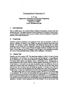
In this paper, aimed at the computational geometry community, we focus on practical algorithms and will only briefly describe the underlying mathematical model given in [11] that relies on recursion theory and domain theory [31, 10, 14]. We have included a succinct introduction to domain theory, recursion theory and the geometric domain in Appendix B. The solid domain (SRd , ⊑) of Rd is the collection of pairs of disjoint open subsets of Rd partially ordered componentwise by subset inclusion: (I, E) ⊑ (I ′ , E ′ ) iff I ⊆ I ′ and E ⊆ E ′ . A classical geometric object, i.e. a subset A ⊆ Rd is represented in this model as (A◦ , (Ac )◦ ), where X ◦ and X c denote respectively the interior and the complement of a set X. More generally, we think of an element (I, E) ∈ SRd as a partial solid or partial geometric objects with interior I, exterior E and boundary (I ∪ E)c . An element (I, E) is maximal in SRd iff I = (E c )◦ and E = (I c )◦ , which imply that I and E are regular 1 . The collection of pairs of interiors of dyadic (or rational) d-polygons forms a basis for SRd . Any partial geometric object (I, E) can be obtained as the union of these basis elements. And (I, E) is computable if there exists an increasing effective sequence of these basis elements with union (I, E). Our new data type is described as follows. We assume that we have lower and upper rational bounds on the coordinates (xk )1≤k≤d of an imprecisely given point x ∈ Rd in say n P given directions, that is we have βj ≤ dk=1 ajk xk ≤ γj , where (ajk )1≤k≤d fixes the n given directions for 1 ≤ j ≤ n. We assume that the set of directions for our data type is known in advance, and is independent from the data itself. Thus, each data point x is located within a rational d-polygon, namely the intersection of the finite number of strips given by the above inequalities. In most applications, we only have the d directions of the coordinate axes, i.e. when each coordinate of an imprecisely given point is known to lie within an interval as in interval analysis, for example when the coordinates of x are given by floating point numbers. But the data type is also essential in cases when we have lower and upper bounds on some linear combination of coordinates. In Figure 1, we have shown 7 out of the 18 possible types of polygons for an imprecisely given point in R2 , where there are precisely three directions 1

An open set is regular if it the interior of its closure

3

of possible approximations: along the two coordinate axes and along the (1, 1) vector, which corresponds to the linear combination x1 + x2 .

Figure 1: Imprecise points defined by three directions (1, 0), (0, 1), (1, 1) Note that the filtered intersection of a non-empty family of convex d-polygons in Rd is a non-empty, convex and compact subset. Our domain of computation is therefore the collection (CRd , ⊇) of all non-empty, convex and compact subsets of Rd ordered by reverse inclusion and equipped with the Scott topology. It is a bounded complete ω-continuous domain (see Appendix B) with a countable basis given by the collection PRd of all rational convex d-polygons in Rd . The map s : Rd → CRd with x 7→ {x} is a topological embedding, i.e. we can identify the maximal elements of this domain with Rd . We also note that (CRd , ⊇) is order isomorphic with a sub-domain of SRd by identifying a non-empty convex and compact set A ∈ CRd with (∅, Ac ) ∈ SRd , i.e. with a geometric object whose interior is empty and its exterior is the complement of A. In subsequent sections, we apply this model of computation to the problem of computing the convex hull, the Delaunay triangulation and the Voronoi diagram of N imprecisely given points in Rd . The partial convex hull is defined as a map of the form H : (CRd )N → SRd , the partial Voronoi diagram as a map of the form V : (CRd )N → (SRd )N and the partial Delaunay triangulation as a map of the form T : (CRd )N → SRd . It will be shown that these maps are Scott continuous and computable; see Appendix B for definitions. In the extended abstract we restrict ourselves to R2 , but the framework and the results here can be extended to Rd in general.

3

Partial Convex Hull

We define the partial convex hull function as a map of the form: H : (CR2 )N C¯

→ SR2 7 → (I, E)

(1)

where C¯ = (C1 , . . . , CN ) represents an ordered list of non-empty convex compact in the plane R2 . The open sets I and E stand for the interior and the exterior of the partial convex hull ¯ In order to define (I, E), we proceed as follows. Let Γ be the classical convex hull map of C. taking a set of points to their convex hull, considered as a compact subset of the plane Γ:

(R2 )N → CR2 P PN (x1 , . . . , xN ) 7→ { N i=1 λi = 1 , λi ≥ 0} i=1 λi xi |

where CR2 is the set of all non-empty compact sets with the Hausdorff metric. For a given ordered list C¯ = (C1 , . . . , CN ) ∈ (CR2 )N of N non-empty compact convex subsets define ¯ = {(p1 , . . . , pN ) | pi ∈ Ci , i = 1, . . . , N } R(C) ¯ An element p ∈ R(C) ¯ to be the set of all possible N -tuples of points, one from each set in C. ¯ is called a representative set of points for C. Now, we formally define (I, E) as:   \ [ (I, E) = ( Γ(p))◦ , ( Γ(p))c  . (2) ¯ p∈R(C)

¯ p∈R(C)

4

c51 d3 d4 d5

d6 (a)

d2 d1

c31 c41

c21 c11 (b)

(c)

(d)

Figure 2: (a) Three given directions have partitioned the unit circle into six arcs; (b) Partial convex hull of five partial points; (c)–(d) Partial convex hull with refined data. Therefore, the exterior of the convex hull of C¯ is the set of points of the plane that are surely not in any of the convex hulls of any representative set of points and the interior is the set of points that are surely in the interior of the convex hull of any representative set of points. ¯ when C¯ ∈ (PR2 )N is an ordered We now develop an N log N algorithm to compute H(C) 2 N list of convex polygons, i.e. a basis element of (CR ) . First, the algorithm to find the exterior comes in two steps: • Obtain the set K of all corners of all the polygons C1 , . . . , CN . • Apply the classical convex hull algorithm to find Γ(K). Since points in the set K have rational coordinates, a computation of Γ(K) using rational arithmetic guarantees a robust and exact algorithm. Computing the interior requires more work. We know that our polygons have been defined by a finite set of directions given, say, by unit vectors d1 , d2 , . . . , dn ordered anticlockwise, where we assume each of these vectors lies in the first or second quadrant, i.e. has nonnegative vertical coordinate. This gives us 2n unit vectors d1 , . . . , dn , dn+1 , . . . , d2n with dn+j = −dj for 1 ≤ j ≤ d \ \ n. Thus, the unit circle is partitioned into a set of 2n arcs dd 1 d2 , d2 d3 , . . . , d2n−1 d2n , d2n d1 . We set d2n+1 := d1 .

Lemma 1 For each polygon Ci (1 ≤ i ≤ N ) and each arc d\ j dj+1 , for 1 ≤ j ≤ 2n there exists a corner cij ∈ Ci , such that for any half plane, with normal ℓ ∈ d\ j dj+1 , containing the polygon Ci , the corner cij is the furthest point of Ci to the boundary of the half plane. Note that in case cij is not unique, we can pick any such corner. Also, we can have cij = cij ′ when j 6= j ′ .

Now that we have a corner cij in the polygon Ci corresponding to the arc d\ j dj+1 , for 1 ≤ j ≤ 2n, we define the interior algorithm as follows: S • For each j = 1, . . . , 2n, obtain the set of rational planar points Kj = 1≤i≤N cij , Lemma 1.

• Apply the classical convex hull algorithm to obtain the convex hull Γ(Kj ) of Kj of corners. T • Compute the intersection I = 1≤j≤2n Γ(Kj ) in rational arithmetic.

Theorem 2 The above algorithms compute the interior and the exterior convex hull.

In the particular case that the partial points are represented by rectangles with sides parallel to coordinate axes, our result is reduced to that in [13]. In fact, in this case, the unit circle in partitioned into the four standard quadrants and ci1 , ci2 , ci3 , and ci4 would be the bottom-left, bottom-right, top-right, and top-left corners of Ci , respectively. Overall, we would then need to compute four classical convex hulls on these sets and take the intersection. Theorem 3 The partial convex hull map H : (CR2 )N → SR2 is Scott continuous and computable with respect to any effective structure on (CR2 )N and any effective structure on SR2 . 5

(a)

(b)

Figure 3: (a) PPB of two polygons, (b) The interior and exterior of a partial disc

4

Partial Perpendicular Bisector

In elementary geometry, a perpendicular bisector of a line segment pq can be defined as the locus of the points on the plane which are neither closer to p nor to q. The perpendicular bisector can be regarded as a partial solid (∅, R2 \ {x : |x − p| = |x − q|}). For a point x ∈ R2 and a compact C ⊂ CR2 , we have the following appropriate distance function. Let ds (x, C) = min{|x − p| : p ∈ C} and dl (x, C) = max{|x − p| : p ∈ C} be, respectively, the shortest and longest distance from x to C. For two compact subsets C1 and C2 , we define the partial Voronoi cell of C1 with respect to C2 as: C12 = {x | dl (x, C1 ) < ds (x, C2 )}

(3)

Similarly we define C21 . The partial perpendicular bisector (PPB) of C1 and C2 is the remaining points of the plane, B(C1 , C2 ) := (C12 ∪ C21 )c = {z ∈ R2 | ∃x ∈ P1 , y ∈ P2 ; |z − x| = |z − y|}, where Ac denotes the complement of A. Note that: \ C12 = {Qx (x, y) | x ∈ P1 , y ∈ P2 )} (4) where Qx (x, y) is the half plane, which contains x and has the perpendicular bisector of xy as its boundary. Thus, C12 is a convex subset. We put δij := ∂Cij . The PBB can be defined as the following Scott continuous and computable map: B : CR2 × CR2 → SR2 (P1 , P2 ) 7→ (∅, C12 ∪ C21 ). Proposition 4 The partial Voronoi cell of a point with respect to a polygon is the intersection of the partial Voronoi cells of the point and the visible edges of the polygon. The partial Voronoi cell of a polygon with respect to another polygon is the intersection of the partial Voronoi cells of each of the vertices of the first polygon with respect to the other polygon. Based on this proposition, we can compute the PPB of two non-intersecting but otherwise arbitrary partial points as in Figure 3(a). Note that if the two partial points intersect, then the PPB will be the whole plane R2 . When the partial points are all rectangles, our construction reduces to that in [25].

6

5

Partial Disc

For three non-collinear points x, y, z ∈ R2 , let Dxyz be the unique closed disc whose boundary circle passes through x, y and z. We extend this definition to partial points. A partial disc is the locus of all discs passing through three points, one from each partial points P1 , P2 and P3 . Formally, we define the partial disc map by: D:

(CR2 )3 → SR2 (P1 , P2 , P3 ) 7→ (DI , DE ),

where DI = DE = ∅ if P1 , P2 and P3 are collinear, i.e. when there exists a straight line T ◦ which intersects P , P and P , otherwise D = ( {D 1 2 3 I xyz | x ∈ P1 , y ∈ P2 , z ∈ P3 }) and S DE = ( {Dxyz | x ∈ P1 , y ∈ P2 , z ∈ P3 })c .

Proposition 5 If P1 , P2 , P3 are non-collinear, O(P1 , P2 , P3 ) = B(P1 , P2 )∩B(P2 , P3 )∩B(P1 , P3 ) will in general be a non-empty hexagon-like compact set whose boundary consists of six vertices and six sides each composed of straight lines and/or parabolic segments from δ12 , δ21 , δ13 , δ31 , δ23 and δ32 , see Figure 3(b). Note that O(P1 , P2 , P3 ) = {s ∈ R2 | ∃x ∈ P1 , y ∈ P2 , z ∈ P3 ; |x − s| = |y − s| = |z − s|}, hence the locus of centers of circles which intersect P1 , P2 and P3 . We call O(P1 , P2 , P3 ) the partial centre of the partial circumcircle of the three partial points. Let D(x, r) denote the closed disc with centre x and radius r. We set oCCF to be the centre of a circle with radius rCCF which passes through (i) the point of P1 closest to oCCF , (ii) the point of P2 closest to oCCF and (iii) the point of P3 furthest from oCCF ; hence the subscript in oCCF . Similarly for the other vertices. Now, consider the three discs D1 = D(oF CC , rF CC ), D2 = D(oCF C , rCF C ) and D3 = D(oCCF , rCCF ) on the one hand and the three discs D1′ = D(oCF F , rCF F ), D2′ = D(oF CF , rF CF ) and D3′ = D(oF F C , rF F C ) on the other hand. Theorem 6 The interior and the exterior of the partial disc are given by:
(DI , DE ) = (D1 ∩ D2 ∩ D3 )◦ , (D1′ ∪ D2′ ∪ D3′ )c .

Theorem 7 The partial disc map D is Scott continuous and computable.

In Figure 3(b), the boundaries of the discs D1 , D2 and D3 are depicted with dotted lines, those of D1′ , D2′ and D3′ with solid lines and the boundaries of the sets DI and DE with dashed lines. The closed region bounded between DI and DE , i.e. bounded between the two closed dashed curves, is called the boundary of the partial disc.

6

Partial Voronoi Diagram

Given a list of N non-empty convex compact subsets C¯ = (C1 , . . . , CN ) ∈ (CR2 )N , the interior of the partial Voronoi cell of Ci is defined to be the set of points which are closer to any point in Ci than to any point in Cj (j 6= i). More precisely, (Vi )I = {x ∈ R2 | ∀j 6= i; dl (x, Ci ) < ds (x, Cj )}. The exterior of the partial Voronoi cell of Ci is defined to be the set (Vi )E = {x ∈ R2 | ∃j 6= i; dl (x, Cj ) < ds (x, Ci )}. Thus, we have \ [ (Vi )I = Cij and (Vi )E = Cji . (5) j6=i

j6=i

We define the partial Voronoi map on a list of N polygons in the plane: V : (CR2 )N → (SR2 )N , 7

with the ith component, 1 ≤ i ≤ N , defined as Vi : C¯ 7→ ((Vi )I , (Vi )E ), where ((Vi )I , (Vi )E ) was defined in Equation 5. We now have: Theorem 8 The partial Voronoi map V : (CR2 )N → (SR2 )N is Scott continuous and computable.

7

Partial Delaunay Triangulation

It is well known that, classically, the computation of the Voronoi diagram of a finite number of points in the plane can be reduced to computing the Delaunay triangulation of these points [7, 16]. We will see that the partial Voronoi diagram of a finite number of partial points can also be computed from a partial Delaunay triangulation of these partial points. Recall that three points of a given set of points in the plane form a Delaunay triangle if and only if their circumcircle does not contain any points of the set in its interior. The centre of the circumcircle is at the intersection point of the PB’s. We will see that in analogy with the classical case, the “partial Delaunay triangulation” of a finite set of partial points in the plane can be computed by determining the “partial discs” of the triples of partial points which do not contain any partial point in their interior. The “partial centre” of the partial disc passing through three partial points is computed by obtaining the intersection of the “PPB’s” of the three “partial edges”. We define a partial edge between two partial points C1 and C2 to be the convex hull of C1 and C2 , written Ed(C1 , C2 ). We can also define a partial triangle to be the partial convex hull of three partial points. Given N partial points C1 , . . . , CN ∈ CR2 , we say that Ed(Ci1 , Ci2 ) is legal if there exists i3 such that for all j 6= i1 , i2 , i3 we have Cj ⊂ DE (Ci1 , Ci2 , Ci3 ), illegal if there exists i3 such that there exists j 6= i1 , i2 , i3 with Cj ⊂ DI (Ci1 , Ci2 , Ci3 ) and indeterminate otherwise. The partial Delaunay triangulation map is now defined as: T :

(CR2 )N → SR2 (C1 , . . . , CN ) 7→ (I, E),

where I = ∅ and [ E = ( {Ed(Ci , Cj ) | Ed(Ci , Cj ) legal or indeterminate})c .

Given any i1 , i2 , i3 , i4 with 1 ≤ i1 , i2 , i3 , i4 ≤ N , we can use the decidable predicate Con in Equation 6 (Appendix B) on dyadic or rational polygons to determine if Ci4 ⊂ DI (Ci1 , Ci2 , Ci3 ) or if Ci4 ⊂ DE (Ci1 , Ci2 , Ci3 ). The following proposition guarantees that flipping an illegal edge makes it legal and vice versa. Proposition 9 Suppose four polygons are given, any three of which satisfy the non-collinearity condition. (i) If one of the polygons intersects the boundary of the partial disc of the other three polygons, then any of the polygons intersects the boundary of the partial disc of the other three polygons. (ii) If one of the polygons is in the interior of the partial disc of the other three polygons, then one of these three polygons is in the exterior of the partial disc of the other three polygons.

8

Now that we have defined partial points, partial edges, partial triangles and partial discs, we apply the classical random incremental algorithm for Delaunay triangulation [7], using Con in Equation 6 instead of the classical predicate for containment of a point in the interior of a disc, for partial objects. This algorithm, as in the classical case, will be N log N on average for non-degenerate data. Note that if the boundary of the partial disc of three polygons intersects other polygons, then the question of legality of the edges between the polygons on the opposite side of the circle remains indeterminate at the present level of precision. Such cases occur in particular whenever a classical degenerate case is approximated, in which the circumcircle of a triangle contains a fourth point on its boundary. While some edges may remain indeterminate at a given stage of computation, the strength of the method lies in detecting those edges which are definitely legal or definitely illegal, so that the right choice can be made. This shows that our model also handles classical degenerate cases. Theorem 10 The partial Delaunay triangulation is Scott continuous and computable. It has to be noted that the map T , although Scott continuous, is not Hausdorff continuous since an indeterminate edge can abruptly disappear with a non-nested perturbation of the input.

References [1] J. P. Aubin and A. Cellina. Differential Inclusions. Springer, 1984. [2] F. Aurenhammer and R. Klein. Voronoi diagrams. In J.-R. Sack and J. Urrutia, editors, Handbook of computational geometry, pages 201–290. Elsevire Science B.V., 1999. [3] F. Avnaim, J. D. Boissonnat, O. Devillers, F. Preparata, and M. Yvinec. Evaluation of a new method to compute signs of determinants. In Proc. Eleventh ACM Symposium on Computational Geometry, June 1995. [4] H. Br¨ onnimann, J. Emiris, V. Pan, and S. Pion. Computing exact geometric predicates using modular arithmetic with single precision. ACM Conference on Computational Geometry, 1997. [5] H. Br¨ onnimann and M. Yvinec. Efficient exact evaluation of signs of determinants. In Proc. Thirteenth ACM Symposium on Computational Geometry, pages 136–173, June 1997. [6] N. J. Cutland. Computability: An Introduction to Recursive Function Theory. Cambridge University Press, 1980. [7] M. de Berg, M. van Kreveld, M. Overmars, and O. Schwarzkopf. Computational geometry, algorithms and applications. Springer, 2nd edition, 2000. [8] H. Desaulniers and N. F. Stewart. Robustness of numerical methods in geometric computation when problem data is uncertain. Computer-Aided Design, special issue on uncertainties in geometrical design, 25(9):539– 545, 1993. [9] O. Devillers, A. Fronville, B. Mourrain, and M. Teillaud. Algebraic methods and arithmetic filtering for exact predicates on circle arcs. In Proc. Sixteenth ACM Symposium on Computational Geometry, pages 139–147, June 2000. [10] A. Edalat. Domains for computation in mathematics, physics and exact real arithmetic. Bulletin of Symbolic Logic, 3(4):401–452, 1997. [11] A. Edalat and A. Lieutier. Foundation of a computable solid modeling. In Proceedings of the fifth symposium on Solid modeling and applications, ACM Symposium on Solid Modeling and Applications, pages 278–284, 1999. [12] A. Edalat and A. Lieutier. Foundation of a computable solid modelling. Theoretical Computer Science, 284(2):319–345, 2002. [13] A. Edalat, A. Lieutier, and E. Kashefi. The convex hull in a new model of computation. In Proc. 13th Canad. Conf. Comput. Geom., pages 93–96, 2001. [14] A. Edalat and P. S¨ underhauf. A domain theoretic approach to computability on the real line. Theoretical Computer Science, 210:73–98, 1998. [15] J. S. Ely and A. P. Leclerc. Correct Delaunay triangulation in the presence of inexact inputs and arithmetic. Reliable Computing, 6:23–38, 2000.

9

[16] S. Fortune. Voronoi diagrams and Delaunay triangulations. In D.-Z. Du and F. Hwang, editors, Computing in Euclidean Geometry, pages 193–233, Singapore, 1992. World Scientific. Lecture notes series on Comput. [17] S. Fortune. Polyhedral modeling with multi-precision integer arithmetic. Computer-Aided Design, 29(2):123– 133, 1997. [18] S. Fortune and C. von Wyk. Efficient exact arithmetic for computational geometry. In Proceeding of the 9th ACM Annual Symposium on Computational Geometry, pages 163–172, 1993. [19] G. Gierz, K. H. Hofmann, K. Keimel, J. D. Lawson, M. Mislove, and D. S. Scott. Continuous Lattices and Domains. Cambrdige University Press, UK, 2003. [20] M. Goodrich, L. Guibas, J. Hershberger, and P. TanenBaum. Snap rounding line segments efficiently in two and three dimensions. In Proc. Thirteenth ACM Symposium on Computational Geometry, pages 284–293, June 1997. [21] L. Guibas, D. Salesin, and J. Stolfi. Epsilon geometry - building robust algorithms for imprecise computations. In Proceeding of the 5th ACM Annual Symposium on Computational Geometry, pages 208–217, 1989. [22] C. Y. Hu, T. Maekawa, E. C. Shebrooke, and N. M. Patrikalakis. Robust interval algorithm for curve intersections. Computer-Aided Design, 28(6/7):495–506, 1996. [23] C. Y. Hu, N. M. Patrikalakis, and X. Ye. Robust interval solid modeling, part ii: boundary evaluation. CAD, 28:819–830, 1996. [24] A. A. Khanban and A. Edalat. Computing Delaunay triangulation with imprecise data. In Proceedings of the 15th Canadian Computational Geometry Conference, 2003. [25] A. A. Khanban, A. Edalat, and A. Lieutier. Computability of partial Delaunay triangulation and Voronoi diagram. Electronic Notes in Theoretical Computer Science, 66(1), 2002. [26] LEDA. http://www.mpi-sb.mpg.de/LEDA/leda.html. [27] V. Milenkovic. Robust polygon modelling. Computer-Aided Design, 25(9), September 1993. [28] R. Moore. Interval Analysis. Prentice-Hall, Englewood Cliffs, 1966. [29] Y. Oishi and K. Sugihara. Topology oriented divide-and-conquer algorithm for Voronoi diagrams. Computer Vision,Graphics, and Image Processing: Graphical Models and Image Processing, 57:303–314, 1995. [30] T. J. Peters, D. R. Ferguson, N. F. Stewart, and P. S. Fussell. Algorithmic tolerances and semantics in data exchange. ACM Conference on Computational Geometry, 1997. [31] M. B. Pour-El and J. I. Richards. Computability in Analysis and Physics. Springer-Verlag, 1988. [32] F. Preparata and M. Shamos. Computational Geometry: an introduction. Springer, 1985. [33] D. S. Scott. Outline of a mathematical theory of computation. In 4th Annual Princeton Conference on Information Sciences and Systems, pages 169–176, 1970. [34] T. W. Sederberg and R. T. Farouki. Approximation by interval Bezier curves. IEEE Comput. Graph. Appl., 15(2):87–95, 1992. [35] M. Segal. Using tolerances to guarantee valid polyhedral modeling results. Computer Graphics, 24(4):105– 114, 1990. [36] K. Sugihara and M. Iri. A robust topology-oriented incremental algorithm for Voronoi diagrams. International Journal of Computational Geometry and Applications, pages 179–228, 1994. [37] K. Sugihara, Y. Ooishi, and T. Imai. Topology-oriented approach to robustness and its application to several Voronoi-diagram algorithms. In Proc. 2nd Canad. Conf. Comput. Geom., pages 36–39, 1990. [38] K. Weihrauch. Computability, volume 9 of EATCS Monographs on Theoretical Computer Science. SpringerVerlag, 1987. [39] C. K. Yap. The exact computation paradigm. In D. Z. Du and F. Hwang, editors, Computing in Euclidean Geometry. World Scientific, 1995. [40] C. K. Yap. Robust geometric computation. In J. E. Goodman and J. O’Rourke, editors, Handbook of Discrete Computational Geometry. CRC Press, 2004.

10

Appendix Part A: Selected Proofs Proof of Theorem 2. The convex hull of a set P of points can be defined as the intersection of all the semi-planes S containing P . Therefore, it is sufficient to prove: \ \ \ \ {S | S is a semi-plane, P ∈ S} = {S | S is a semi-plane, Kj ∈ S}, ¯ P ∈R(C)

1≤j≤2n

where Kj = {c1j , . . . , cN j }, as in Lemma 1. It is easy to see that the RHS contains the LHS. To prove the other way, we show that for every semi-plane S in the LHS, there exists an S ′ in the RHS such that S ′ ⊆ S. One can easily see that if S contains at least one point of each partial point, then it must contain a corner of each. Lemma 1 shows that S contains cij in each partial point, where j depends on the direction of the normal to the boundary of S. So, we choose the semi-plane S ′ to be the intersection of all semi-planes containing cij with the same direction as of S. Since S ′ is in the RHS, the proof is complete. The convex hull map of a compact set is defined as: ˆ : (CRd ) → CRd Γ where CRd is the set of all non-empty compact subsets of Rd with the Hausdorff metric, and CRd is the set of all non-empty compact convex subsets of Rd with the Hausdorff metric. ˆ is non-expansive with respect to the Hausdorff metric. i.e. dH (Γ(A), ˆ ˆ Theorem 11 The map Γ Γ(B)) ≤ dH (A, B), and therefore Hausdorff continuous. ˆ ˆ Proof. Assume dH (Γ(A), Γ(B)) > r. Without loss of generality we can assume that: ˆ ˆ ∃a ∈ Γ(A), s.t. b(a, r) ∩ Γ(B) = ∅, ˆ where b(a, r) is a ball with centre a and radius r. Because both b(a, r) and Γ(B) are convex, there is a plane separating them, that is: ˆ ∃s ∈ S d−1 , u ∈ R : Γ(B) ⊂ {x | s · x − u ≤ 0} b(a, r) ⊂ {x | s · x − u ≥ 0} ⇒ a ∈ {x | s · x − u − r ≥ 0} ˆ ⇒ Γ(A) 6⊂ {x | s · x − u − r ≤ 0}

(1)

(2)

We can easily see that: (1) ⇒ B ⊂ {x | s · x − u ≤ 0} (2) ⇒ A 6⊂ {x | s · x − u − r ≤ 0}



⇒ dH (A, B) > r,

which proves the Theorem. Lemma 12 Suppose A is a closed regular compact set, then we have: ∀ǫ > 0, ∃δ > 0, A ⊂ (A−δ ) where,

+ǫ

X +ǫ = {y | d(y, X) < ǫ}, X −ǫ = {y | d(y, cl(X c )) > ǫ}.

11

Proof. For any set A,

S

−δ δ>0 A

= A◦ . Also, for any regular set A and ǫ > 0:

∀x ∈ A, ∃y ∈ A◦ .d(x, y) < ǫ (regularity) y ∈ A◦ ⇒ ∃δ > 0.y ∈ A−δ +ǫ ⇒ x ∈ (A−δ )

which proves A⊂

[

+ǫ

(A−δ )

δ>0 +ǫ

A is compact, therefore ∃δ > 0, s.t. A ⊂ (A−δ ) . Proposition 13 Suppose A, A′ , B, and B ′ are compact and A ∩ B and A′ ∩ B ′ are regular 2 . Then ∀ǫ > 0, ∃δ > 0, such that dH (A, A′ ) < δ

&

dH (B, B ′ ) < δ ⇒ (A′ ∩ B ′ )+ǫ ⊃ (A ∩ B)

&

(A ∩ B)+ǫ ⊃ (A′ ∩ B ′ )

i.e. dH ((A ∩ B), (A′ ∩ B ′ )) < ǫ. Proof. We prove (A′ ∩ B ′ )+ǫ ⊃ (A ∩ B). The other relation is proved in the same way. ) −δ dH (A, A′ ) < δ ⇒ A ⊂ A′ +δ ⇒ A−δ ⊂ (A′ +δ ) ⇒ −δ A is compact ⇒ (A′ +δ ) = A′◦ ⇒ A−δ ⊂ A′ ⇒ (A ∩ B)−δ ⊂ A′ . Similarly for B, we have (A ∩ B)−δ ⊂ B ′ . So, (A ∩ B)−δ ⊂ (A′ ∩ B ′ ). Using Lemma 12, we +ǫ have (A ∩ B) ⊂ [(A ∩ B)−δ ] . Combining these two gives: (A′ ∩ B ′ )+ǫ ⊃ (A ∩ B). Corollary 14 The classical convex hull map Γ is non-expansive with respect to the Hausdorff metric. i.e. dH (Γ(A), Γ(B)) ≤ dH (A, B), and therefore Hausdorff continuous. T Corollary 15 The two maps HI : (CR2 )N → CR with (C1 , . . . CN ) 7→ p∈R(C) ¯ Γ(p) and S 2 N HE : (CR ) → CR with (C1 , . . . CN ) 7→ p∈R(C) ¯ Γ(p) are Hausdorff continuous.

Proof of Theorem 3. Since H is clearly monotone, it follows by Corollary 15 that it is Scott continuous. Suppose P¯ ∈ (PR2 )N is a basis element and let (O1 , O2 ) ∈ SR2 be a basis element of SR2 , where O1 and O2 are interiors of two disjoint rational polygons. Then the relation (O1 , O2 ) ≪ H(P¯ ), which is equivalent to cl(O1 ) ⊂ HI (P¯ ) and cl(O2 ) ⊂ HE (P¯ ) is decidable since O1 , O2 , HI (P¯ ), HE (P¯ ) are four rational polygons. It follows that, given effective structures on (CR2 )N and SR2 , the set {< m, n > |bm ≪ H(an )} is recursive, where (an )n∈ω and (bm )m∈ω are the enumerations of the basis elements of (CR2 )N and SR2 respectively, and the result follows.

Proof of Proposition 5 (outline). We prove that under the non-collinearity assumption δ12 ∩ δ13 is a singleton, namely oF CC . Then we show that the intersection δ12 ∩ δ32 is unique and happens somewhere between oF CC and any point of δ12 ∩ δ31 on δ12 . Note that δ12 ∩ δ31 is not necessarily unique and can be empty. This ensures that the shape of the partial centre is hexagon-like. Proof of Theorem 6 (outline). We prove that no circle whose centre is inside the partial centre can take part in building the boundary. Among those circles with centres on the boundary of the partial centre, we prove that only those on the six corners of the hexagon-like region can contribute to the boundary of the partial disc. It is then easy to see that the interior is built up from the intersection of those discs which pass through the closest point of two of the partial points and the furthest point of the third partial point. The exterior is built up from the union of the other three discs. 2

A closed subset is regular if it is the closure of its interior

12

Part B: Domain theory and Recursion theory We give here the formal definitions of a number of notions in domain theory used in the paper; see [19, 31] for more detail. We think of a partially ordered set (poset) (P, ⊑) as the set of output of some computation such that the partial order is an order of information: in other words, a ⊑ b indicates that a has less information than b. For example, the set {0, 1}∞ of all finite and infinite sequences of bits 0 and 1 with a ⊑ b if the sequence a is an initial segment of the sequence b is a poset and a ⊑ b simply means that b has more bits of information than a. A non-empty subset A ⊆ P is directed if for any pair of elements a, b ∈ A there exists c ∈ A such that a ⊑ c and b ⊑ c. A directed set is therefore a consistent set of output elements of a computation: for every pair of output a and b, there is some output c with more information than a and b. An increasing sequence is the simplest example of a directed set in P . A directed complete partial order (dcpo) or a domain is a partial order in which every directed subset F A ⊆ P has a least upper bound (lub) denoted by A. If a domain has a least element then it is denoted by ⊥ and called bottom. For two elements a and b of a dcpo we sayFa is way-below or approximates b, denoted by a ≪ b, if for every directed subset A with b ⊑ A there exists c ∈ A with a ⊑ c. The idea is that a is a finitary approximation to b: whenever the lub of a consistent set of output elements has more information than b, then already one of the input elements in the consistent set has more information than a. In {0, 1}∞ , we have a ≪ b iff a ⊑ b and a is a finite sequence. The closed subsets of the Scott topology of a domain are those subsets C which are downward closed (i.e. x ∈ C & y ⊑ x ⇒ y ∈ C) F and closed under taking lubs of directed subsets (i.e. for every directed subset A ⊆ C we have A ∈ C). A basis of a domain D is a subset B ⊆ D such that for every element x ∈ D of the domain F the set Bx = {y ∈ B|y ≪ x} of elements in the basis way-below x is directed with x = Bx . An (ω)-continuous domain is a dcpo with a (countable) basis. In other words, every element of a continuous domain can be expressed as the lub of the directed set of basis elements which approximate it. In a continuous dcpo D, subsets of the form ↑a = {x ∈ D|a ≪ x}, for a ∈ D, forms a basis for the Scott topology. A domain is bounded complete if every bounded subset has a lub; in such a domain every non-empty subset has an infimum or greatest lower bound. It can be shown that a function f : D → E between dcpo’s is continuous with respect to the Scott topology if and only if it is monotone (i.e. a ⊑ b F⇒ f (a) ⊑ F f (b)) and preserves lubs of directed sets i.e. for any directed A ⊆ D, we have f ( a∈A a) = a∈A f (a). Moreover, if D is an ω-continuous dcpo, F then f is Fcontinuous iff it is monotone and preserves lubs of increasing sequences (i.e. f ( i∈ω xi ) = i∈ω f (xi ), for any increasing (xi )i∈ω ). Thus, it is enough to compute f on basis elements to obtain an algorithm that computes approximations which converge to f (x) for any x The interval domain (I[0, 1]n , ⊇) of the unit box [0, 1]n ⊆ Rn is the set of all non-empty n-dimensional sub-rectangles in [0, 1]n ordered by reverse inclusion, i.e. A ⊑ B iff A ⊇ B; it is a bounded complete ω-continuous domain, with A ≪ B iff A◦ ⊃ B. A basic Scott open set is given, for every open subset O of Rn , by the collection of all rectangles contained in O. The map x 7→ {x} : [0, 1]n → I[0, 1]n is an embedding onto the set of maximal elements of I[0, 1]n . Every maximal element {x} can be obtained as the least upper bound (lub) of an increasing chain of elements, i.e. a shrinking, nested sequence of sub-rectangles, each containing {x} in its interior and thereby giving an approximation to {x} or equivalently to x. The set of sub-rectangles with rational coordinates or with dyadic coordinates provides a countable basis. One can similarly define, for example, the interval domain IRn of Rn . The domain (CRd , ⊇) of all non-empty convex and compact subsets of Rd is a bounded complete ω-continuous domains with A ≪ B iff A◦ ⊃ B and a countable basis consisting of all rational convex d-polygons. The domain (SRd , ⊑) of all disjoint pains of open subsets of Rd ordered componentwise by subset inclusion (i.e. (A1 , A2 ) ⊑ (B1 , B2 ) iff A1 ⊆ B1 and A2 ⊆ B2 ) is a bounded complete ω-continuous domain

13

with (A1 , A2 ) ≪ (B1 , B2 ) iff the closures cl(A1 ) and cl(A2 ) are compact subsets of B1 and B2 respectively. An ω-continuous domain D with a least element ⊥ is effectively given wrt an effective enumeration b : N → B of a countable basis B if the set {< m, n > |bm ≪ bn } is recursive, where < ., . >: N × N → N is the standard pairing function i.e. the isomorphism (x, y) 7→ (x+y)(x+y+1) + x. This means that for each pair of basis elements (bm , bn ), it is possible to 2 decide in finite time whether or not bm ≪ bn . We say x ∈ D is computable if the set {n|bn ≪ x} is r.e. This is equivalent to say that there is a master programme which outputs exactly this set. It is also equivalent to theFexistence of a recursive function g such that (bg(n) )n∈ω is an increasing chain in D with x = n∈ω bg(n) . We can define an effective enumeration ξ of the set Dc of all computable elements of D. Let θn , n ∈ ω, be the nth partial recursive function. It can be F shown [14] that there exists a total recursive function σ such that ξ : N → Dc with ξn := i∈ω bθσ(n) (i) , with (bθσ(n) (i) )i∈ω an increasing chain for each n ∈ ω, is an effective enumeration of Dc . A sequence (xi )i∈ω is computable if there exists a total recursive function h such that xi = ξh(i) for all i ∈ ω. We say that a continuous map f : D → E of effectively given ω-continuous domains D (with basis {a0 , a1 , . . .}) and E (with basis {b0 , b1 , . . .}) is computable if the set {< m, n > |bm ≪ f (an )} is r.e. This is equivalent to say that f maps computable sequences to computable sequences. Computable functions are stable under change to a recursively equivalent basis. Every computable function can be shown to be a continuous function [38, Theorem 3.6.16]. It can be shown [14] that these notions of computability for the domain IR of intervals of R induce the same class of computable real numbers and computable real functions as in the classical theory [31]. An important feature of domains, in the context of this paper, is that they can be used to obtain computable approximations to operations which are classically non-computable. For example, comparison of a real number with 0 is not computable. However, the function N : I[−1, 1] → {tt, ff}⊥ with   tt if b < 0 N ([a, b]) = ff if 0 < a  ⊥ otherwise is the computable approximation to the comparison predicate.3 Here, {tt, ff}⊥ is the three element pointed domain with two incomparable maximal elements tt and ff. Also the containment predicate defined by the authors in [25], has been used in Delaunay triangulation algorithm in this paper: Con : CR2 × (CR2 )3 → {+, −}⊥   tt if C ⊂ I(C1 , C2 , C3 ) (C, (C1 , C2 , C3 )) 7→ ff if C ⊂ E(C1 , C2 , C3 )  ⊥ otherwise.

(6)

It has been shown in [25] that Con is Scott continuous and is decidable on basis elements, which means that if the input (C, (C1 , C2 , C3 )) is a tuple of dyadic (or rational) polygons, then we can decide in finite time if Con is true or false for this input, i.e. containment in the interior and exterior of the partial circle is semi-decidable.

3

In this paper, we assume a machine model of computation a RAM (Random Access Memory) machine able to perform usual integer (and hence rational and dyadic) arithmetic. As regards computability, this machine model is equivalent to a universal Turing machine.

14