INTERNATIONAL JOURNAL OF COMPUTERS COMMUNICATIONS & CONTROL ISSN 1841-9836, 12(3), 365-380, June 2017.
Computational Intelligence-based PM2.5 Air Pollution Forecasting M. Oprea, S.F. Mihalache, M. Popescu Mihaela Oprea*, Sanda Florentina Mihalache, Marian Popescu Automatic Control, Computers and Electronics Department Petroleum-Gas University of Ploieşti Romania, 100680 Ploieşti, Bd. Bucureşti, 39 {mihaela, sfrancu, mpopescu}@upg-ploiesti.ro *Corresponding author:
[email protected] Abstract: Computational intelligence based forecasting approaches proved to be more efficient in real time air pollution forecasting systems than the deterministic ones that are currently applied. Our research main goal is to identify the computational intelligence model that is more proper to real time PM2.5 air pollutant forecasting in urban areas. Starting from the study presented in [27]a , in this paper we first perform a comparative study between the most accurate computational intelligence models that were used for particulate matter (fraction PM2.5 ) air pollution forecasting: artificial neural networks (ANNs) and adaptive neuro-fuzzy inference system (ANFIS). Based on the obtained experimental results, we make a comprehensive analysis of best ANN architecture identification. The experiments were realized on datasets from the AirBase databases with PM2.5 concentration hourly measurements. The statistical parameters that were computed are mean absolute error, root mean square error, index of agreement and correlation coefficient. Keywords: computational intelligence, PM2.5 air pollution forecasting, ANFIS, ANN, ANN architecture identification. Reprinted (partial) and extended, with permission based on License Number 3957050363449 [2016] ©IEEE, from "Computers Communications and Control (ICCCC), 2016 6th International Conference on". a
1
Introduction
This paper is an extension of [27] (doi: 10.1109/ICCCC.2016.7496746). A comprehensive comparative study is here presented. In addition, an extended analysis for the identification of best neural network architecture is included. We report our new experimental results. Air pollution forecasting is an important research topic especially for the improvement of life quality in cities. Among currently used forecasting methods, computational intelligence methods proved to be more efficient in real time forecasting systems. The deterministic methods which take into account many variables related to the forecasted parameter and use a precise mathematical model with embedded physical and chemical factors (e.g. those based on climate models) give better solutions, but in a longer period of time. In contrast, computational intelligence based methods are approximate methods, that give solutions with a good forecasting accuracy, in short periods of time. Thus, the real time forecasting systems used for urban population early warning of air pollution episodes occurrence can be based on computational intelligence techniques. Artificial intelligence (AI) provides several techniques for building forecasting systems, mainly from its computational intelligence part and less from its symbolic part. Such applications in different domains were reported in the literature, most of them in the economic, energy and environmental fields [1], [18], [25]. Symbolic AI is used as a knowledge based approach in selecting some important parameters that influence the forecasting systems performance, usually for the prediction model features selection. On the other hand, computational intelligence techniques Copyright © 2006-2017 by CCC Publications
366
M. Oprea, S.F. Mihalache, M. Popescu
can be used as effective predictors’ builders (see e.g. [5], [12], [16], [29], [30]). An important environmental problem that needs better solutions nowadays is urban air quality improvement and reducing human health effects due to air pollution in cities. For this, good real time air pollution short-term forecasters have to be developed and included in the environmental management systems or in the early warning system of intelligent environmental decision support systems. Particulate matter with diameter less than 2.5 µm (PM2.5 ) is an air pollutant that has potential negative effects on human health, when its concentration exceeds the admissible standard upper level. Our research work focuses on the development of a good real time PM2.5 air pollution forecasting model that will be integrated in the ROKIDAIR Decision Support System (ROKIDAIR DSS) to be used in two pilot Romanian cities, Ploieşti and Târgovişte, by the ROKIDAIR Early Warning System. Starting from a literature review and a comparative study between most used computational intelligence based forecasting methods, we have selected the best model which is a neural network model and we have performed an analysis of best neural network architecture identification via trial and error method. Computational intelligence is a paradigm introduced in [2] which combines mainly three computing technologies: fuzzy computing, neural computing and evolutionary computing. Fuzzy computing and neural computing are used as forecasting models, while evolutionary computing can be applied mainly for the optimization of a forecasting model. In the last decade, other nature-inspired computing methods were added to computational intelligence, such as swarm intelligence with various techniques: ant colony optimization (ACO), particle swarm intelligence (PSO), artificial bee colony algorithm (ABC) etc. These last techniques are commonly used for optimizing the forecasting model and not as a forecasting model. The remainder of the paper is organized as follows. In Section 2 it is described computational intelligence based forecasting focusing on most used techniques: artificial neural networks and adaptive neuro-fuzzy inference system (ANFIS). A comparative study of the two techniques (ANN and ANFIS) applied to PM2.5 air pollution forecasting is presented in Section 3, concluding that the best experimental results were obtained by the ANN forecasting model. The identification of the best PM2.5 ANN forecasting architecture is discussed in Section 4. The final section concludes the paper and highlights some future work.
2
Computational intelligence based forecasting
Computational intelligence provides data-driven methods. The neural methods applicable to solve forecasting problems are: artificial neural network (ANN) and adaptive neuro-fuzzy inference system (ANFIS). They can perform air pollution forecasting more efficiently than the deterministic methods by capturing the knowledge accumulated in the historical data sets (time series) which is learned via a training algorithm and is used to accurately predict specific air pollution parameters (e.g. air pollutants concentrations).
2.1
Artificial Neural Networks (ANN)
Artificial neural networks are universal approximators of non-linear functions [14]. They are composed by a number of non-linear processing units named artificial neurons which are structured in layers. Forecasting problems are solved mainly by feed-forward ANNs (multi-layer perceptron - MLP and radial basis function - RBF) and recurrent ANNs. Figure 1 shows the general architecture of a feed-forward ANN, which has an input layer, some hidden layers and an output layer.
Computational Intelligence-based PM2.5 Air Pollution Forecasting
input layer
hidden layers
367
output layer
W11
Inp1
W12 W1m
Inp2
. . .
. . .
. . .
. . .
. . .
Out1
. . . Outn
Inpm
Figure 1: The general architecture of a feed-forward ANN A recurrent neural network is a type of artificial neural network that has a directed cycle made by the connections between the artificial neurons, allowing it to have an internal state. Thus, it exhibits a dynamic behaviour which provides the ability to process and predict chaotic time series for long-terms [19]. A recurrent ANN is an ANN that has feedback, allowing arbitrary connections between neurons, both forward and backward (i.e. recurrent). Thus, it propagates data bi-directional, from input to output and from output to input. Recurrent ANNs are universal approximators [34]. They provide a very good performance in temporal structures modeling, as well as in real world problem solving ( [4], [6]). Recurrent ANNS exhibit a dynamic temporal behavior and can process arbitrary sequences of inputs (e.g. chaotic time series). The best structure of an ANN is experimentally determined. Usually, a single hidden layer is enough to capture the nonlinearity of any function. Deep networks are ANNs with several hidden layers. The number of hidden nodes is chosen by experiments, while the number of input and output nodes is set according to the forecasting problem that has to be solved. The number of input nodes represents the input window (in the case of time series, the number of past hours measurements) and the number of output nodes represents the forecast horizon (number of future time steps, hours, days etc., for which the prediction is determined). The ANN is trained with a training set (which is extracted from a data set) by using a specific training algorithm (the most used being backpropagation and the Levenberg-Marquardt algorithm), after that following the validation and testing steps which are executed on the validation set and testing set, respectively. Details on the ANN computational algorithms are given in the literature (see e.g. [13]). The Levenberg Marquardt algorithm [20] is an iterative algorithm that estimates the weights vector of the ANN model by minimizing the sum of the squares of the deviation between predicted and target values. If ANN training is too long then overfitting can occur. To avoid this, the ANN training is stopped earlier, as soon as the performance on testing data is not improved any more.
2.2
ANFIS
The ANFIS method applied to prediction uses a hybrid architecture composed by a fuzzy inference system FIS enhanced with ANN features proposed by Jang [15]. The advantages of FIS are mainly its design that emulates human thinking and the simple interpretation of the results. Integrating the ANN part into a fuzzy inference system enhanced the FIS part with learning/adapting capabilities. The prediction model does not use a mathematical model as well as the case of ANN. The ANFIS architecture has the structure given in Figure 2.
368
M. Oprea, S.F. Mihalache, M. Popescu
Training and validating data ANN
Knowledge base
Input Membership functions
Rule weight
FIS structure
Output Membership functions
FIS
Inputs Testing data
Fuzzification
Fuzzy Inference Engine
Defuzzification
Forecasted Output
Figure 2: The general architecture of ANFIS The FIS part is formed by five functional units: a fuzzification unit (from crisp value to fuzzy set), a defuzzification unit (from fuzzy set to a crisp value), the database unit (containing the description of membership functions for input/output variables), a rule base unit (all the rules defined for FIS), and the decision unit (performing the inference operations on the fuzzy rules) [26]. The neuro-fuzzy architecture is capable to learn new rules or membership functions, to optimize the existing ones (Figure 2). The training data determine restrictions on the design methods for the rule base and membership functions. Usually the particular type of datasets for PM2.5 eliminates the subclustering method in generating the FIS structure, a good choice being the grid partition method. The ANFIS architecture (Figure 2) has five layers, with Takagi-Sugeno rules. The first layer (adaptive) forms the premise parameters (the IF part with inputs and their membership functions). The second layer computes a product of the involved membership functions. The third layer normalizes the sum of inputs. In layer 4, the adaptive i-node computes the contribution of i-th rule to ANFIS output, forming the consequence parameters (the THEN part with output and its membership function). The fifth layer makes the summation of all inputs. The ANN part can improve the membership functions associated with FIS structure. Usually these membership functions are the tuning parameters of the FIS. Their initial values are chosen from experience or trial and error methods. In the training mode the ANN finds the most suited membership functions for the input-output relation described by FIS, according to training and checking dataset. ANFIS applies a hybrid learning algorithm (H) or backpropagation (BP) algorithm. The hybrid learning algorithm identifies premise parameters with gradient method and consequence parameters with least square method. At feedforward propagation step from H, the system output reaches layer 4, and the consequence parameters are formed with least square method. With backpropagation (BP) optimization method, the error signal is fed back and the new premise parameters are computed through gradient method. The prediction method is tested with datasets that respect the main features of training dataset. The prediction precision decreases with enlarging the prediction window from one hour in advance to six hours in advance.
2.3
An overview on PM2.5 computational intelligence based forecasting
The main computational intelligence techniques that were used for PM2.5 forecasting are: feed forward ANN, radial basis function ANN, recurrent ANN, and ANFIS. Other AI techniques such as genetic algorithms and swarm intelligence were applied to optimize the forecasting model. We have selected some PM2.5 forecasting systems based on computational intelligence that were
Computational Intelligence-based PM2.5 Air Pollution Forecasting
369
reported in the literature. In the first years of the current century, the PM2.5 forecasting ANN models (usually, of MLP type) were compared mostly with statistical models such as linear regression, ARMA, ARIMA, revealing a very good performance of the neural models. One of the earlier PM2.5 forecasting neural models were proposed in [21] and [31]. The first ANN model was applied in Canada, while the latter was applied in Santiago de Chile. The experimental results described in both papers showed a very good performance of the ANN model in comparison with the traditional statistical models (e.g. linear regression). In the next years, various comparisons between different types of ANNs models used to PM2.5 forecasting were performed. For example, an analysis of three ANN models (MLP, RBF-ANN and square MLP) applied to PM2.5 short term prediction in an area on the US-Mexico border is presented in [28]. The experimental results revealed that for the analyzed area the RBF-ANN model outperformed the other two models. Another work that analyzes the performance of different neural network models and regression model applied to forecasting expressway fine PM (i.e. PM2.5 ) in Indiana, USA is described in [35]. A feed forward ANN with backpropagation training algorithm is described in [?], for 3 days in advance forecasting of PM10 , SO2 and CO air pollutants (AP) levels in the Besiktas district in Istanbul, Turkey. The ANN is integrated in the AirPol system (http://airpol.fatih.edu.tr). The ANN inputs are daily meteorological forecasts and the AP indicator values. The authors applied some geographical models, the most complex one being based on the distance between two sites in the case of using three selected neighborhood districts. In [10] it is demonstrated the efficacy of using EnviNNet, a prototype stochastic ANN model for air quality forecasting in cities from Italy (Rome, Milan and Napoli) to predict PM10 in Phoenix, Arizona in comparison with the use of CMAQ system. The ANN is a MLP that uses the conjugate-gradient method for training. In the last years, the research work was focused on combining PM2.5 forecasting ANN models with other techniques, such as statistical techniques, data mining, genetic algorithms, wavelet transformation, deep learning, that can improve the forecasting accuracy. Some examples are briefly described as follows. A research work that reports the successful use of ANNs and principal component analysis for PM10 and PM2.5 forecasting in two cities, Thessaloniki (Greece) and Helsinki (Finland) is described in [36]. The authors used a MLP and the meteorological and AQ pollutants to predict the next day mean concentration of PM10 and PM2.5 . A genetically optimized ANN and k-means clustering was applied in [8] to predict PM10 and PM2.5 in a coastal location of New Zealand. A hybrid PM2.5 forecasting model that uses feed forward ANN combined with rolling mechanism and accumulated generating operation of gray model, that was experimented in three cities from China is introduced in [11]. Another recent work on PM2.5 neural forecasting is described in [9]. The authors propose a novel hybrid model that combines air mass trajectory analysis with wavelet transformation in order to improve the accuracy of the average PM2.5 concentration two days in advance neural forecasting. The ANN is a MLP trained with a backpropagation algorithm and the Levenberg-Marquardt (LM) algorithm. Also, early stopping was used to avoid overfitting. Some meteorological parameters were used. Finally, one of the newest achievements for PM2.5 prediction in 52 cities from Japan is reported in [24]. Each city has several thousands of PM2.5 sensors. A deep recurrent neural network (DRNN) is proposed for PM2.5 prediction based on real data sensors, which applies a novel pre-training method (DynPT) using time series prediction especially designed auto-encoder. The experimental results showed that the DRNN model outperformed the current climate models used in Japan, which are based on Eulerian and Lagrangian grids or Trajectory models. The use of pure FIS for specific air pollutants is reported in literature. In [3] it is presented a study for Mexico City air pollution. The paper present a solution of classifying different air
370
M. Oprea, S.F. Mihalache, M. Popescu
parameters via fuzzy reasoning and include this solution in the air quality index calculation. In [7] it is formulated a fuzzy based forecasting model used in Polish Environmental Agency, a model that forecast specific air pollutants based on decades of measurements. Examples of ANFIS based systems for the prediction of air pollutants concentrations are presented in [22], [23], [32] and [33]]. In [23] it is proposed a fuzzy inference system to forecast PM2.5 concentrations at specific hours using as additional input the medium temperature. In [33] it is developed a fuzzy inference system to forecast ozone concentrations levels based on other pollutants and meteorological parameters. The provided FIS model accuracy has the best values for coefficient of determination. For the city of Konya, Turkey the literature present the solution of ANFIS forecasting model for PM10 trained with large datasets [32]. In [22] there are presented three case studies from three different cities from Romania. Each time the proposed ANFIS forecasting model for PM10 is tested and there are made recommendations on how to adjust the model parameters to improve forecasting accuracy. The main conclusion of the literature overview is that an efficient PM2.5 forecasting ANN model can be derived only by experiment, depending on the PM2.5 measurements data sets and several characteristics (climatic, geographic, industrial, economic, social etc) specific to the analyzed area. Thus, there is no pre-set ANN model type for PM2.5 that is proper for any area. Another important conclusion is that both ANN and ANFIS can model non-linear time series.
3 3.1
A Comparative study of PM2.5 forecasting with ANFIS and ANN Data sets PM2.5(t-3) PM2.5(t-2) PM2.5(t-1)
ANFIS / ANN forecasting model
PM2.5(t+1)
PM2.5(t)
Figure 3: Structure of the proposed architecture For this study were chosen two urban traffic PM2.5 monitoring stations. Taking into consideration the lack of data for the Romanian stations, the data used for training and validation were from a München (Germany) station where sufficient data are available (4 years) in the Airbase database. In addition, the testing was done using also data (from 2015) from Ploieşti (Romania), a city which presents interest as part of a larger project (ROKIDAIR project- www.rokidair.ro). The data set from München contains 34000 samples and the PM2.5 hourly concentration has a range of 0.52-168.5 µg/m3 . The additional testing data from Ploieşti contains 4000 samples and the domain of PM2.5 concentration is 3.24-36.45 µg/m3 . The data were normalized and then divided (randomly) as follows: 70% for training, 15% for validation and 15% for testing the model. If the amount of data is large enough, it is supposed that the data contains the effect of other pollutants and meteorological data, so the proposed architecture (Figure 3) for the forecasting
Computational Intelligence-based PM2.5 Air Pollution Forecasting
371
model (ANFIS or ANN) has as inputs the values of PM2.5 concentrations from current hour to three hours ago and as output the prediction for the next hour. In order to determine the suitability of the models the following statistical parameters were calculated: MAE - mean absolute error; RMSE - root mean square error; IA - index of agreement; R - correlation coefficient. The two errors measure how close the predicted data are to the true values and have to be as small as possible, and the last two indices are numbers that indicate how well the data fit the prediction model and they should be close to 1. The experiments presented in the following sections were performed using MATLAB© environment.
3.2
Experimental results for ANFIS model
In this study, for the generation of the fuzzy inference system was used the grid partition method, imposed by the specific of data. The membership functions were triangular and Gaussian and the optimization algorithms of the ANN were backpropagation and hybrid. The ANFIS model was tested for all combinations between the modifiable parameters, namely the membership functions types and the optimization methods. Table 1 presents the experimental results of the ANFIS model tested with data from München. Table 1: Statistical indices for ANFIS model (München) ANFIS Structure Trimf/Hybrid Gauss/Hybrid Trimf/Backprop. Gauss/Backprop.
MAE [µg/m3 ] 1.9614 1.9419 2.0494 2.2177
RMSE [µg/m3 ] 3.2564 3.2089 3.3933 3.4471
IA 0.9796 0.9801 0.9778 0.9770
R 0.9604 0.9616 0.9573 0.9556
Analyzing Table 1 it can be seen that the best configuration is when a Gaussian function is used for the membership functions associated to inputs, and for the training of the neural network a hybrid algorithm is used. In this case, the RMSE is the smallest, and the IA and R have the biggest values. The smallest training and validation errors are around 0.02. The best configuration of the ANFIS structure was also tested with data from the Ploieşti station. The values of the statistical parameters are presented as follows: MAE [µg/m3 ]: 1.0166; RMSE [µg/m3 ]: 1.9160; IA: 0.9711; R: 0.9447.
3.3
Experimental results for ANN model
The structure of the neural network contains four neurons in the input layer, one hidden layer and one neuron in the output layer. There were used two types of neural networks, namely feed forward backpropagation (FF) and layer recurrent (LR), with Levenberg-Marquardt as training algorithm, and the adaptive learning functions were gradient descent with momentum weight and bias (learngdm - LGDM ) and gradient descent weight and bias (learngd - LGD). The simulations were performed modifying also the number of neurons in the hidden layer (from three to twelve). The training and validation errors are with two orders of magnitude smaller than the ones obtained in the case of ANFIS model, with values around 0.0004. In Table 2 is presented a selection with the values of the statistical parameters for the ANN models. The best configurations of the ANN models are highlighted, being associated to the
372
M. Oprea, S.F. Mihalache, M. Popescu
layer recurrent structure with 4 neurons in the hidden layer and the learngd adaptation learning function, and the feedforward structure with 5 neurons in the hidden layer and the learngdm adaptation learning function, respectively. In this case the mean absolute error and the root mean squared error have the smallest values, and IA and R indices have the biggest values. Table 2: Statistical indices for ANN model with one hidden layer (München) ANN Structure FF 4x4x1/LGDM LR FF 4x4x1/LGD LR FF 4x5x1/LGDM LR FF 4x5x1/LGD LR FF 4x6x1/LGDM LR FF 4x6x1/LGD LR FF 4x7x1/LGDM LR FF 4x7x1/LGD LR FF 4x8x1/LGDM LR FF 4x8x1/LGD LR FF 4x10x1/LGDM LR FF 4x10x1/LGD LR
MAE [µg/m3 ] 1.9421 1.9683 1.9421 1.9278 1.9340 1.9836 1.9609 1.9486 1.9415 1.9676 1.9471 1.9519 1.9402 1.9528 1.9489 1.9567 1.9516 1.9498 1.9433 1.9613 1.9657 1.9527 1.9568 1.9791
RMSE [µg/m3 ] 3.2086 3.2359 3.2086 3.1931 3.1966 3.2360 3.2152 3.2138 3.2149 3.2207 3.2292 3.2182 3.2185 3.2252 3.2128 3.2224 3.2218 3.2130 3.2148 3.2290 3.2272 3.2183 3.2167 3.2367
IA 0.9802 0.9798 0.9802 0.9804 0.9804 0.9797 0.9800 0.9801 0.9801 0.9800 0.9799 0.9801 0.9801 0.9800 0.9801 0.9800 0.9800 0.9801 0.9801 0.9799 0.9799 0.9800 0.9800 0.9797
R 0.9616 0.9609 0.9616 0.9619 0.9619 0.9609 0.9614 0.9614 0.9614 0.9613 0.9611 0.9613 0.9613 0.9612 0.9615 0.9612 0.9612 0.9615 0.9614 0.9611 0.9611 0.9613 0.9614 0.9609
In addition, as in the ANFIS case, the best configurations of the RNN and FFNN structure were tested with data from the Ploieşti station and the values of the statistical parameters from Table 3 were obtained. Table 3: Statistical indices for ANN model (Ploieşti) RNN FFNN
MAE [µg/m3 ] 0.9672 0.9852
RMSE [µg/m3 ] 1.3713 1.3970
IA 0.9852 0.9846
R 0.9714 0.9702
The experimental results confirms that the best ANN configuration (RNN) previously obtained provides very good results for the testing data set from Ploieşti.
Computational Intelligence-based PM2.5 Air Pollution Forecasting
3.4
373
Discussion
A comparison between the best values of the statistical parameters obtained for the ANFIS model and the ANN models, respectively, using München datasets is synthesized in Table 4. Table 4: Comparison between best results Forecasting Method Best ANFIS Best RNN Best FFNN
MAE [µg/m3 ] 1.9419 1.9278 1.9340
RMSE [µg/m3 ] 3.2089 3.1931 3.1966
IA 0.9801 0.9804 0.9804
R 0.9616 0.9619 0.9619
It can be observed that the results obtained with ANN are slightly better than the ANFIS results, and corroborated with the fact that for Ploieşti data the statistical indices are much better in the case of ANN (see sections 3.2 and 3.3) and the time for training is much smaller (with at least 10 times) for ANN, it can be concluded that the ANN forecasting model is most suitable for the prediction of PM2.5 concentrations. Therefore, in the next section the focus will be on the ANN forecasting model.
4
Best ANN architecture identification for PM2.5 forecasting
Usually, an ANN with one hidden layer is enough for any complex nonlinear function (see e.g. [37]). However, in order to make a complete analysis, several ANN architectures with one hidden layer and two hidden layers were experimented. Thus, the selected architectures (RNN and FFNN) with one hidden layer from the previous section were tested with two hidden layers. Also, different adaptive learning functions were used: gradient descent with momentum weight and bias and gradient descent weight and bias, and different number of neurons in the second hidden layer (from three to twelve). A trial and error method was applied in order to identify the best ANN forecasting model architecture. The best ANN architecture selection was determined using the same statistical indices as in the section 3. It is interesting to analyze how is influenced the forecasting accuracy (error) of the ANN model by the number of hidden layers and the number of hidden neurons in each hidden layer. More hidden layers involve a deeper learning ability of the ANN model. However, the number of hidden layers is dependent on the application specific data sets (e.g. in our case PM2.5 concentration hourly measurements) and must be determined by experiment until optimum prediction (i.e. minimum RMSE). Table 5 presents a selection of the statistical indices values for an ANN architecture with two hidden layers, which has four neurons in the first hidden layer and 3 to 12 neurons in the second hidden layer.
374
M. Oprea, S.F. Mihalache, M. Popescu Table 5: Statistical indices for ANN model with two hidden layers (München)) ANN Structure FF 4x4x4x1/LGDM LR FF 4x4x4x1/LGD LR FF 4x4x5x1/LGDM LR FF 4x4x5x1/LGD LR FF 4x4x7x1/LGDM LR FF 4x4x7x1/LGD LR FF 4x4x8x1/LGDM LR FF 4x4x8x1/LGD LR FF 4x4x9x1/LGDM LR FF 4x4x9x1/LGD LR FF 4x4x10x1/LGDM LR FF 4x4x10x1/LGD LR
MAE [µg/m3 ] 1.9319 1.9491 1.9303 1.9338 1.9397 1.9494 1.9475 1.9491 1.9460 1.9776 1.9291 1.9102 1.9562 1.9428 1.9472 1.9320 1.9350 1.9310 1.9353 1.9630 1.9359 1.9481 1.9377 1.9516
RMSE [µg/m3 ] 3.2041 3.2159 3.1923 3.2120 3.2065 3.2228 3.2192 3.2258 3.2292 3.2450 3.2028 3.1890 3.2264 3.2356 3.2131 3.2061 3.2149 3.2062 3.2165 3.2346 3.2105 3.2137 3.2149 3.2327
IA 0.9803 0.9801 0.9804 0.9802 0.9802 0.9800 0.9801 0.9800 0.9800 0.9796 0.9803 0.9805 0.9799 0.9800 0.9801 0.9803 0.9801 0.9802 0.9801 0.9799 0.9802 0.9801 0.9802 0.9799
R 0.9617 0.9614 0.9620 0.9615 0.9616 0.9612 0.9613 0.9612 0.9611 0.9607 0.9617 0.9621 0.9611 0.9610 0.9615 0.9617 0.9314 0.9616 0.9614 0.9609 0.9615 0.9615 0.9614 0.9610
Changing the number of neurons in the first hidden layer from 4 to 5 the results from Table 6 are obtained. The number of neurons in the second hidden layer is the same as in the previous case (from 3 to 12 neurons).
Computational Intelligence-based PM2.5 Air Pollution Forecasting
375
Table 6: Statistical indices for ANN model with two hidden layers (München) ANN Structure FF 4x5x4x1/LGDM LR FF 4x5x4x1/LGD LR FF 4x5x5x1/LGDM LR FF 4x5x5x1/LGD LR FF 4x5x7x1/LGDM LR FF 4x5x7x1/LGD LR FF 4x5x8x1/LGDM LR FF 4x5x8x1/LGD LR FF 4x5x9x1/LGDM LR FF 4x5x9x1/LGD LR FF 4x5x10x1/LGDM LR FF 4x5x10x1/LGD LR
MAE [µg/m3 ] 1.9455 1.9491 1.9512 1.9338 1.9627 1.9489 1.9389 1.9835 1.9313 1.9556 1.9314 1.9791 1.9256 1.9350 1.9380 1.9446 1.9505 1.9184 1.9181 1.9658 1.9336 1.9429 1.9164 1.9441
RMSE [µg/m3 ] 3.2076 3.2159 3.2137 3.2120 3.2302 3.2265 3.2012 3.2450 3.2147 3.2257 3.1957 3.2499 3.1926 3.1961 3.2025 3.2249 3.2251 3.1926 3.1678 3.2414 3.2041 3.2145 3.2053 3.2136
IA 0.9802 0.9801 0.9801 0.9802 0.9799 0.9799 0.9802 0.9796 0.9802 0.9799 0.9804 0.9796 0.9804 0.9803 0.9803 0.9800 0.9800 0.9804 0.9807 0.9797 0.9802 0.9801 0.9803 0.9801
R 0.9616 0.9614 0.9614 0.9615 0.9610 0.9611 0.9617 0.9607 0.9614 0.9612 0.9619 0.9606 0.9620 0.9619 0.9617 0.9612 0.9612 0.9620 0.9626 0.9608 0.9617 0.9614 0.9617 0.9614
Analyzing the results from Tables 5 and 6 it can be observed that the best ANN architecture with two hidden layers is feedforward with five neurons in the first hidden layer, nine neurons in the second hidden layer and gradient descent weight and bias as the adaptive learning function (Figure 4). In this case, MAE and RMSE have the smallest values and IA and R have the biggest values.
Figure 4: Best ANN architecture
For the best architecture mentioned above are presented in Figures 5 and 6 the testing error evolution and a partial view of the comparison between testing and forecasted data for München data set.
376
M. Oprea, S.F. Mihalache, M. Popescu
0.4 0.3
Testing error
0.2 0.1 0 -0.1 -0.2 -0.3 -0.4 0
1000
2000
3000
4000
5000
Samples
Figure 5: Testing error for best ANN architecture (FF - 4x5x9x1)
0.22 Testing data Forecasting data
0.2 0.18
Data
0.16 0.14 0.12 0.1 0.08 0.06 0.04 4100
4150
4200
4250
4300
4350
4400
Samples
Figure 6: Comparison of testing vs forecasted data for best ANN architecture (FF - 4x5x9x1)
Table 7: Best ANN Architecture Best ANN architecture with one hidden layer with two hidden layers
MAE [µg/m3 ] 1.9278 1.9181
RMSE [µg/m3 ] 3.1931 3.1678
IA 0.9804 0.9807
R 0.9619 0.9626
Table 7 concludes that using an ANN architecture with two hidden layers improves the results obtained with the ANN architecture one hidden layer suggesting a possible use of this type of structure for PM2.5 forecasting.
Computational Intelligence-based PM2.5 Air Pollution Forecasting
5
377
Conclusions and future works
This paper is an extension of [27] which proposed PM2.5 air pollution forecasting models based on computational intelligence techniques. Starting from the study presented in [27], in this paper we extend the comparative study between artificial neural networks (ANNs) and adaptive neurofuzzy inference system (ANFIS) which are the most accurate computational intelligence models used for particulate matter (fraction PM2.5 ) air pollution forecasting by increasing the number of neurons in the hidden layer of the ANN architecture. We also present an extended overview of computational intelligence techniques based on neural networks approach with up to date solutions of air pollution forecasting. The data used for training and validation were from a München (Germany) urban traffic station available from the Airbase database with hourly PM2.5 concentrations (for 4 years). For the testing of the model data from Ploieşti (Romania), a city which presents interest as part of a larger project (ROKIDAIR project - www.rokidair.ro) were also used. The proposed models have four PM2.5 hourly concentrations as inputs and the prediction of the next hour PM2.5 concentration. We compared the performances of the models using statistical indices such as mean absolute error, root mean square error, index of agreement and correlation coefficient. The simulation results obtained with ANN are better than the ANFIS results, and corroborated with the fact that for Ploieşti data the statistical indices are much better in the case of ANN and the time for training is much smaller (with at least 10 times) for ANN, it can be concluded that the ANN forecasting model is most suitable for the prediction of PM2.5 concentrations. Therefore, the next part of the paper concentrates on finding the best neural network architecture by increasing the number of hidden layer of the ANN architecture. In this new approach there are performed numerous simulations with different architectures starting from the best architectures with one hidden layer obtained in Section 3. Therefore we kept the number of the neurons in the first hidden layer and varied the number of neurons in the second different layers. The paper proposes an ANN model for PM2.5 forecasting, whose architecture was identified via trial and error method, during an extended analysis that was performed. The simulation results pointed out that introducing another hidden layer is beneficial in terms of statistical indices that assess the forecasting performance. This is a good premise to find other solutions using deep learning as future work. The model can be used to real time forecasting and is incorporated in the ROKIDAIR DSS, being used by the ROKIDAIR Early Warning System in case some PM2.5 air pollution episodes arise in different areas from the two pilot cities: Ploieşsti and Târgovişte. The selection of the most proper computational intelligence based PM2.5 forecasting model was made during the comprehensive comparative study of applying the ANN and ANFIS models, which proved to be efficient in real time forecasting systems. The ANN PM2.5 forecasting model can detect concentrations above the standard limit values for the human health protection. As future work we will extend the study for the improvement of the forecasting model performance through deep learning or combining neural networks with wavelets or data mining techniques.
Acknowledgment The research leading to these results has received funding from EEA Financial Mechanism 2009-2014 under the project ROKIDAIR "Towards a better protection of children against air pollution threats in the urban areas of Romania" contract no. 20SEE/30.06.2014.
378
M. Oprea, S.F. Mihalache, M. Popescu
Bibliography [1] Alfaro M.D.; Sepúlveda J.M.; Ulloa J.A. (2013); Forecasting Chaotic Series in Manufacturing Systems by Vector Support Machine Regression and Neural Networks, International Journal of Computers Communications & Control, ISSN 1841-9836, 8(1), 8-17, 2013. [2] Bezdek J.C. (1994); What is computational intelligence?, Computational Intelligence - Imitating Life, IEEE World Congress on Computational Intelligence (WCCI), ISBN: 9780780311046, 1-12, 1994. [3] Carbajal-Hernández J.J.; Sánchez-Fernández L.P.; Carrasco-Ochoa J.A.; Martínez-Trinidad J.F. (2012); Assessment and prediction of air quality using fuzzy logic and autoregressive models, Atmospheric Environment, 60, 37-50, 2013. [4] Cherif A.; Cardot H.; Boné R. (2011); SOM time series clustering and prediction with recurrent neural networks, Neurocomputing, ISSN: 0925-2312, 74(11), 1936-1944, 2011. [5] Cherkassky V., Krasnopolsky V.; Solomatine D.P., Valdes J. (2006); Computational intelligence in earth sciences and environmental applications: Issues and challenges, Neural Networks, 19, 113-121, 2006. [6] Connor J.T., Martin R., Atlas L.E. (1994); Recurrent neural networks and robust time series prediction, IEEE Transactions on Neural Networks, 5(2), 240-254, 1994. [7] Domańska D., Wojtylak M. (2012); Application of fuzzy time series models for forecasting pollution concentrations, Expert Systems with Applications, 39, 7673-7679, 2012. [8] Elangasinghe M.A.; Singhal N.; Dirks K.N.; Salmond J.A.; Samarasinghe S. (2014); Complex time series analysis of PM10 and PM2.5 for a coastal site using artificial neural network modeling and k-means clustering, Atmospheric Environment, 94, 106-116, 2014. [9] Feng X.; Li Q.; Zhu Y.; Hou J.; Jin L.; Wang J. (2015); Artificial neural networks forecasting of PM2.5 pollution using air mass trajectory based geographic model and wavelet transformation, Atmospheric Environment, 107, 118-128, 2015. [10] Fernando H.J.S., Mammarella M.C., Grandoni G., Fedele P., Di Marco R.; Dimitrova R., Hyde P. (2012); Forecasting PM10 in metropolitan areas: Efficacy of neural network, Environmental Pollution, ISSN 0269-7491, 163, 62-67, 2012. [11] Fu M., Wang W., Le Z., Khorram M.S. (2015); Prediction of particulate matter concentrations by developed feed-forward neural network with rolling mechanism and gray model, Neural Computing & Applications, 26(8), 1789-1797, 2015. [12] Gardner M.W., Dorling S.R. (1998); Artificial neural networks (the multilayer perceptron) - a review of applications in the atmospheric sciences, Atmospheric Environment, 32, 26272636, 1998. [13] Hertz J., Krogh A., Palmer R.G. (1991); Introduction to the theory of neural computation, Addison Wesley, ISBN: 978-0201515602, 1991. [14] Hornik K., Stinchcombe M., White H. (1989); Multilayer feedforward networks are universal approximators, Neural Networks, 2, 356-366, 1989. [15] Jang R. (1993); ANFIS: Adaptive-Network-Based Fuzzy Inference System, IEEE Transactions on Systems, Man and Cybernetics, 23(3), 665-685, 1995.
Computational Intelligence-based PM2.5 Air Pollution Forecasting
379
[16] Karatzas K.D., Voukantsis D. (2008); Studying and predicting quality of life atmospheric parameters with the aid of computational intelligence methods, International Congress on Environmental Modelling and Software (iEMS), 2, 1133-1139, 2008. [17] Kumar Chandar S., Sumathi M., Sivanadam S.N. (2016); Forecasting Gold Prices Based on Extreme Learning Machine, International Journal of Computers Communications & Control, ISSN 1841-9836, 11(3), 372-380, 2016. [18] Kurt A., Oktay A.B. (2010); Forecasting air pollutant indicator levels with geographic models 3 days in advance using neural networks, Expert Systems with Applications, 37, 7986-7992, 2010. [19] Mandic D., Chambers J. (2001); Recurrent Neural Networks for Prediction: Learning Algorithms, Architectures and Stability, ISBN: 978-0-471-49517-8, Wiley, 2001. [20] Marquardt D. (1963); An algorithm for least squares estimation of nonlinear parameters, SIAM Journal of Applied Mathematics, ISSN: 0036-1399, 11, 431-441, 1963. [21] McKendry I.G. (2002); Evaluation of artificial neural networks for fine particulate pollution (PM10 and PM2.5 ) forecasting, Journal of the Air & Waste Management Association, 52, 1096-1101, 2002. [22] Mihalache S.F., Popescu M.; Oprea M. (2015); Particulate Matter Prediction using ANFIS Modelling Techniques, Proc. of 19th International Conference on System Theory, Control and Computing (ICSTCC), October 14-16, Cheile Gradistei, Romania, ISBN: 978-1-47998481-7, 895-900, 2015. [23] Nebot A., Mugica F. (2014); Small-Particle Pollution Modeling Using Fuzzy Approaches, M.S. Obaidat et al. (eds.), Simulation and Modeling Methodologies, Technologies and Applications, Advances in Intelligent Systems and Computing, ISBN: 978-3-319-03580-2, Springer International Publ. 239-252, 2014. [24] Ong B.T., Sugiura K., Zettsu K. (2016); Dynamically pre-trained deep recurrent neural networks using environmental monitoring data for predicting PM2.5 , Neural Computing & Applications, ISSN: 1433-3058, 27, 1553-1566, 2016. [25] Oprea M., Buruiana V., Matei A. (2010); A Microcontroller-based Intelligent System for Real-time Flood Alerting, International Journal of Computers Communications & Control, ISSN 1841-9836, 5(5), 844-851, 2010. [26] Oprea M.; Dragomir E.G.; Mihalache S.F.; Popescu M. (2014); Prediction methods and techniques for PM2.5 concentration in urban environment (in Romanian), S. Iordache and D. Dunea (eds.), Methods to assess the effects of air pollution with particulate matter on children’s health (in Romanian), MatrixRom, ISBN: 978-606-25-0121-1, 387-428, 2014. [27] Oprea M.; Mihalache S.F., Popescu M. (2016); A comparative study of computational intelligence techniques applied to PM2.5 air pollution forecasting, Computers Communications and Control (ICCCC), 2016 6th International Conference on, ISBN: 978-1-5090-1735-5, 103-108, 2016. [28] Ordieres J.B., Vergara E.P., Capuz R.S., Salazar R.E. (2005); Neural network prediction model for fine particulate matter (PM2.5 ) on the US-Mexico border in El Paso (Texas) and Ciudad Juárez (Chihuahua), Environmental Modelling & Software, ISSN: 1364-8152, 20, 547-559, 2005.
380
M. Oprea, S.F. Mihalache, M. Popescu
[29] Palit A.K., Popovic D. (2005); Computational Intelligence in Time Series Forecasting Theory and Engineering Applications, Springer, ISBN 978-1-85233-948-7, 2005. [30] Pasero E., Mesin L. (2010); Artificial Neural Networks to Forecast Air Pollution, In: Air Pollution, Vanda Villanyi (Ed.), InTech, ISBN: 978-953-307-143-5, 221-240, 2010. [31] Peréz P., Trier A., Reyes J. (2000); Prediction of PM2.5 concentrations several hours in advance using neural networks in Santiago, Chile, Atmospheric Environment, ISSN 13522310, 34, 1189-1196, 2000. [32] Polat K., Durduran S.S. (2012); Usage of output-dependent data scaling in modeling and prediction of air pollution daily concentration values (PM10 ) in the city of Konya, Neural Computing and Applications, ISSN: 1433-3058, 21, 2153-2162, 2012. [33] Savić M., Mihajlović I., Arsić M., Živković Z. (2014); Adaptive-network-based fuzzy inference system (ANFIS) model-based prediction of the surface ozone concentration, Journal of the Serbian Chemical Society, ISSN 1820-7421, 79(10), 1323-1334, 2014. [34] Schäfer A.M., Zimmermann H.-G. (2006); Recurrent neural networks are universal approximators, ICANN, 16th International Conference, Proceedings, ISBN 978-3-540-38627-8, 1, 632-640, 2006. [35] Thomas S., Jacko R.B. (2007); Model for forecasting expressway fine particulate matter and carbon monoxide concentration: application of regression and neural network model, Journal of Air Waste Management Association, ISSN: 2162-2906, 57(4), 480-488, 2007. [36] Voukantsis D.; Karatzas K.; Kukkonen J.; Räsänen T.; Karppinen A.; Kolehmainen M. (2011); Intercomparison of air quality data using principal component analysis and forecasting of PM10 and PM2.5 concentrations using artificial neural networks, in Thessaloniki and Helsinki, Science of the Total Environment, ISSN: 0048-9697, 409, 1266-1276, 2011. [37] Zhang G., Patuwo B.E.; Hu M.Y. (1998); Forecasting with artificial neural networks: the state of the art, International Journal of Forecasting, ISSN: 0169-2070, 14(1), 35-62, 1998.