Computational Models of Learning the Raising-Control Distinction

Res on Lang and Comput DOI 10.1007/s11168-011-9073-6

Computational Models of Learning the Raising-Control Distinction William Garrett Mitchener · Misha Becker

© Springer Science+Business Media B.V. 2011

Abstract We consider the task of learning three verb classes: raising (e.g., seem), control (e.g., try) and ambiguous verbs that can be used either way (e.g., begin). These verbs occur in sentences with similar surface forms, but have distinct syntactic and semantic properties. They present a conundrum because it would seem that their meaning must be known to infer their syntax, and that their syntax must be known to infer their meaning. Previous research with human speakers pointed to the usefulness of two cues found in sentences containing these verbs: animacy of the sentence subject and eventivity of the predicate embedded under the main verb. We apply a variety of algorithms to this classification problem to determine whether the primary linguistic data is sufficiently rich in this kind of information to enable children to resolve the conundrum, and whether this information can be extracted in a way that reflects distinctive features of child language acquisition. The input consists of counts of how often various verbs occur with animate subjects and eventive predicates in two corpora of naturalistic speech, one adult-directed and the other child-directed. Proportions of the semantic frames are insufficient. A Bayesian attachment model designed for a related language learning task does not work well at all. A hierarchical Bayesian model (HBM) gives significantly better results. We also develop and test a saturating accumulator that can successfully distinguish the three classes of verbs. Since the HBM and saturating accumulator are successful at the classification task using biologically

W. G. Mitchener (B) Department of Mathematics, College of Charleston, Robert Scott Small Building, Room 339, 175 Calhoun St., Charleston, SC 29424, USA e-mail: [email protected] M. Becker Linguistics Department, University of North Carolina, 301 Smith Building, CB#3155, Chapel Hill, NC 27599-3155, USA e-mail: [email protected]

123

W. G. Mitchener, M. Becker

realistic calculations, we conclude that there is sufficient information given subject animacy and predicate eventivity to bootstrap the process of learning the syntax and semantics of these verbs. Keywords Bayesian inference · Child language acquisition · Clustering · Control · Raising · Syntax · Unsupervised learning 1 Introduction One of the fundamental problems in language learning is that of determining the hierarchical structure that underlies a given sentence string. Closely related is the problem of deducing meanings of verbs, especially abstract verbs, as verbs’ lexical meanings are entangled with syntax (Gleitman 1990; Fisher et al. 1991; Lidz et al. 2004; Levin and Rappaport Hovav 2005, among many others). That is, the meaning of a verb is intimately related to the type of argument structure the verb participates in, and so being able to categorize verbs according to their semantic argument-taking properties should go hand-in-hand with understanding the syntax of the sentence strings. In this paper, we discuss the case of distinguishing raising verbs (e.g. seem) from control verbs (e.g. try). Raising and control verbs overlap in one of the sentential environments they occur in (John seemed/tried to be nice). Although the verb classes are partially distinguishable by occurrence in certain other environments, the presence of a class of ambiguous verbs (verbs that can be either raising or control) significantly complicates the learning problem because the “distinguishing” environments do not actually give unambiguous information about category membership (Becker 2005b, 2006). Rather, based on psycholinguistic evidence we argue that learners can exploit semantic information within the overlapping environment to categorize a novel verb as raising or control (Becker and Estigarribia 2010). Here we focus on the problem of discriminating the verb classes, with the assumption that knowing which class a verb belongs to will allow the learner to determine the structure of the otherwise ambiguous string.1 To give a brief preview, we investigate learning models that attempt to classify a verb as raising, control, or ambiguous, from sample sentences of the surface form (1) John likes to run Subject Main- verb to Predicate If the main verb is a control verb, the subject of such a sentence is the semantic subject of both the main verb and the predicate (John is the “liker” and the “runner”). If the main verb is a raising verb, the subject is semantically related only to the predicate, and is raised to the subject position of the sentence to satisfy the requirement that English 1 We frame the learning problem in terms of the construction of verb types, and the categorization is done on the basis of encountering tokens of verbs. We could have framed it, instead, in terms of assigning a binary category to each token encountered. However, since ultimately learners must have a categorical representation of types, we chose to frame the problem in the former way. Framing the process in this way underscores the parallel between this specific learning process and other categorization processes that children must undertake in learning language (types of grammatical categories, subcategories of verbs, etc.).

123

Computational Models of Learning the Raising-Control Distinction

sentences must have a syntactic subject. If the argument structure of a verb is known (that is, it is known whether the verb requires, allows, or forbids a semantic subject), then the underlying syntax of the sentence is easily deduced. However, raising and control verbs have rather abstract meanings in that they add information to another predicate, and one wonders how children could infer their argument structure without some knowledge of the underlying syntax. Thus, the acquisition of the syntax and semantics of these verbs poses something of a chicken-and-egg problem. Although surface word order-type information in such sentences is insufficient to determine which class the main verb belongs to, basic semantic information about the subject (whether it is animate or inanimate) and predicate (whether it is eventive or stative) is available. Control verbs as a class prefer animate subjects and eventive predicates because many of their uses have to do with intentions or preferences concerning an action. Raising verbs have less of a preference because many of their meanings are tense-like or convey uncertainty, and can apply to a wider set of predicates. In this article, we investigate the possibility that such basic semantic information suffices to bootstrap the acquisition process. We will focus on how a learner could determine whether an unknown verb is of the raising, ambiguous, or control class; specifically, whether it forbids, allows, or requires a semantic subject. After providing additional linguistic background, we discuss data sets drawn from the CHILDES and Switchboard corpora, in which sentences using various raising, control, and ambiguous verbs have been collected and marked for subject animacy and predicate eventivity. In the following sections we develop learning models that use probabilistic tendencies in the input to approximate the way in which actual language learners might acquire the raising, control, and ambiguous verb classes over time. We apply several learning algorithms to this data and the problem of classifying or clustering the verbs into the appropriate classes. A huge variety of potentially useful algorithms exist, including classifiers, Bayesian inference, ranking, and clustering. Each requires input in a different format and yields its own particular kind of output. The intent of the project is not to determine which of these algorithms works best. There is no shootout to be won or lost, and we will not attempt to resolve all the issues of how to fairly compare them. Rather, we are interested in resolving the conundrum of how children begin to acquire raising and control syntax and semantics: Does the primary linguistic data contain information that is accessible to children who do not yet have a complete grasp of their native language, and is sufficient for beginning to infer which verbs fall into which class? Do any of these algorithms indicate that subject animacy and predicate eventivity provide sufficient information accessible through a computation that the human brain could likely be performing? Are any of them consistent with the pattern of acquisition and use of these verbs observed in children? Many of the algorithms do work fairly well, indicating that despite all the complications, enough basic semantic information is present in the data to bootstrap the process of learning the syntax and semantics of raising, control, and ambiguous verbs. The hierarchical Bayesian model described in Sect. 4.1.3 is especially successful at classifying these verbs, but it is unclear whether its behavior is consistent with child language. The new accumulator algorithm described in Sect. 4.2 classifies most of

123


the verbs by analyzing sentences sequentially, and it reproduces certain properties of child language. 2 Linguistic and Psycholinguistic Background Both raising and control verbs can occur in the string in (2). (2) Scott to paint with oils. a. Scotti tends [ti to paint with oils] (raising) b. Scotti likes [PROi to paint with oils] (control) The primary difference between the two constructions is that in the control sentence there is a thematic (semantic, selectional) relationship between the main verb and the subject, while in the raising sentence there is no such relation: the subject of the sentence is thematically related only to the lower predicate (paint with oils). Thus, the string in (2) represents a case where, until the learner has acquired the syntactic and semantic properties of the main verb, the learner cannot simply take a string of input and immediately deduce the correct underlying structure. Since what distinguishes the two structures is the main verb’s category, we see the verb categorization task as the first step in solving the parsing problem. There are other types of sentence frames that partially distinguish these classes of verbs. For instance, control verbs cannot occur with an expletive (semantically empty) subject (e.g. it, there), while raising verbs can. This is because control verbs assign a θ -role to their subject, and expletives cannot bear a θ -role (Chomsky 1981). (3) There tend to be arguments at poker games. (4) *There like to be arguments at poker games. Some control verbs, but no raising verbs, can occur in transitive or intransitive frames.2,3 (5) John likes bananas. (6) *John tends bananas. (7) *John hopes bananas. Note that not all control verbs can be transitive, as in (7). Some raising verbs can occur with a subordinate clause, but this is not possible with every raising verb, and not with any control verbs: (8) It seems that John is late. (9) *It tends that John is late. (10) *It hates that John is late. 2 The raising verbs tend and happen have homophonous forms that are (in)transitive, e.g. John tends sheep,

or Interesting things happened yesterday. The general problem of homophony is significant for learning but is beyond the scope of this paper. 3 Verbs in this frame could also be non-control transitive or intransitive verbs, like eat; of interest here are verbs that could occur in both a transitive/intransitive frame and a frame with an infinitive complement. We ignore here the further problem that transitive or intransitive verbs can occur with an adjunct infinitive clause, as in John runs to stay in shape.

123


Taking a naïve view of the learning procedure one might hypothesize that, since only control verbs are banned from sentences like (3), a learner should assume, given a novel verb in a sentence like (2), that the novel verb is a control verb. This is a “subset” type of approach, since the assumption is that the set of constructions that control verbs occur in form a subset of the set of constructions that raising verbs occur in. If the learner has guessed incorrectly, she will eventually encounter an input sentence like (3), and this datum would provide the triggering evidence to change her grammar. Furthermore, if the learner has guessed correctly, she might have data such as (5) to confirm her categorization of the verb. However, we contend that such a strategy is insufficient for three reasons explained below. The first argument is based on the existence of verbs that are ambiguous between having a raising or a control interpretation, including begin, start, continue and need. As discussed by Perlmutter (1970) these verbs can occur in raising contexts (e.g., with an expletive subject), but they can also have a control interpretation when they occur with an animate subject. (11) It began to rain. (raising) (12) There began to be more and more ants. (raising) (13) Rodney began to talk to Zoe. (control) Moreover, ambiguous verbs also occur in single clause frames as transitive or intransitive verbs. (14) The game began at 3 o’clock. (15) The referee started the match. Since ambiguous verbs can occur in all of the environments that both raising and control verbs can, their existence raises a challenge for language learners. Begin will be heard with an expletive subject, as in (11), where it will be analyzed as a raising verb, and it will be heard with an animate subject as in (13), where it should be analyzed as a control verb. But tend, which is unambiguously raising, will also be heard with expletive subjects (3) and animate subjects (Scott tends to paint with oils). In the absence of explicit negative evidence (Chomsky 1959; Marcus 1993) how will a learner determine that tend is not ambiguous and therefore does not function as a control verb when it occurs with an animate subject? The learner will not encounter *Scott tends oil paint. Furthermore, if the learner needed to hear a verb used transitively in order to classify it as control, certain control verbs would be categorized incorrectly since they do not occur in a transitive frame (e.g. hope). The second argument against the subset strategy is that in speech to children, raising verbs occur disproportionately more frequently in the ambiguous surface frame (2) than in disambiguating environments, such as with an expletive subject (Hirsch and Wexler 2007). Therefore, presumably learners will need to at least make a guess about the category of a verb encountered in this sentence frame prior to encountering the verb in other frames. The third argument is that previous experimental research has shown that adult speakers make use of two types of cues from within the ambiguous surface frame (2) to make a guess about whether a given ambiguous string is likely to be a raising or a control sentence. These cues come from whether the subject is animate or inanimate

123


(see (16a–b)) and whether the predicate inside the infinitive clause is stative or eventive (see (17a–b)). (16) a. b. (17) a. b.

Samantha likes to be tall. (animate) The tower seems to be tall. (inanimate) Samantha hates to mow the lawn. (eventive) Samantha seems to be happy. (stative)

The evidence comes from a psycholinguistic experiment in which adults were asked to fill in the main verb in an incomplete sentence (Becker 2005a). The properties of subject animacy and predicate eventivity were systematically manipulated. Participants gave significantly more control verbs when the sentence had an animate subject or an eventive lower predicate, and they gave significantly more raising verbs when the sentence had an inanimate subject or a stative lower predicate. While these cues indicate tendencies for these verb classes (not definitive restrictions; cf. Samantha hates to be tall), the psycholinguistic data show that they are very strong tendencies. A further psycholinguistic study with adults (Becker and Estigarribia 2010) showed that speakers are highly sensitive to the cue of subject animacy in making a guess about whether a novel verb is of the raising or the control class. In a word learning study, adult participants were presented with novel verbs with only animate subjects or with at least one inanimate subject. When verbs were presented with only animate subjects, adults were strongly biased to categorize novel verbs as control verbs. However, presentation of a novel verb with at least one inanimate subject significantly overrode their bias and led adults to categorize the novel verb as a raising verb. Thus, speakers do appear to draw inferences about a verb’s category when encountered in the ambiguous frame (2), and we believe child learners are likely to make use of this information as well. In fact, there is empirical evidence that this is so. For example, when the subject of the sentence is inanimate, 3- and 4-year-olds interpret a verb in the frame in (2) as if it were a raising verb, even if it is actually a control verb in the adult grammar (Becker 2006). In brief, there is information in the ambiguous sentence frame that can aid a learner in distinguishing the classes of raising and control verbs, and there is psycholinguistic evidence that speakers make use of this information. In Sect. 4.2, we describe a new on-line classification algorithm that was designed to start in a neutral state and be able to assign a verb to a more restrictive or a less restrictive class after sufficient data has been collected, in contrast to subset learning algorithms which can only move to less restrictive hypotheses. That children permit verbs of one class to behave like verbs from the other class early on will become relevant in evaluating our proposed algorithm, as it mimics this early neutral stance on categorization. Future work should include an extension into the use of cross-sentential cues in verb learning. 3 Description of Data We have searched two sources of naturalistic spoken language. The Switchboard corpus (Taylor et al. 2003) contains naturalistic adult-to-adult speech recorded in phone conversations. The CHILDES database (MacWhinney 2000) contains dozens of

123

Computational Models of Learning the Raising-Control Distinction Table 1 Mothers’ distribution of raising verbs Verb

Animate + eventive

Animate + stative

Inanimate + eventive

Inanimate + stative 5

Seem

0

4

1

Used

32

13

2

3

Going

1065

132

31

27

Total

1097

149

34

88% eventive

35 49% eventive

corpora of speech to children, much of it recorded in spontaneous conversations between parents or researchers and young children. 3.1 CHILDES Due to the need for handcoding of the CHILDES data, our dataset of child-directed speech is somewhat limited in size. We analyzed the mothers’ speech (the *MOT tier) in all of the Adam, Eve and Sarah files within the Brown (1973) corpus. The total number of *MOT utterances in the Brown corpus is over 59,500. We began by searching for all occurrences of specific raising, control and ambiguous verbs followed by the word to, using the CLAN program.4 Each utterance in the output was then coded by hand by Becker for whether the subject was animate or inanimate, and whether the predicate inside the infinitive phrase was eventive or stative. Cases in which the subject was null were counted if it was clear from the context what the referent of the subject was. For example, Adam’s mother’s question “Want to give this to Ursula?” was clearly directed at Adam (“(Do you) want to …”) and so it was counted as having an (implied) animate subject. Utterances in which the lower predicate was elided or unclear were not counted. The total number of utterances excluded because the predicate was unclear or elided was: 7 control (e.g. I don’t want to), 9 raising (e.g. It doesn’t seem to), and 1 ambiguous (Now she’s starting to …); hence, a relatively small proportion of the overall counts. Subject animacy was judged according to whether the referent was living or nonliving (also whether it would be replaced with a he/she pronoun or it pronoun, with the exception that insects would likely be referred to with it but are alive). Predicate eventivity was judged according to whether the predicate typically occurs in the present progressive with an on-going meaning (these are eventive: e.g., John is walking) or whether it occurs in the simple present tense with an on-going (i.e. non-habitual) meaning (these are stative: e.g., John knows French). The results, summing across the three children’s mothers, are given in Tables 1, 2 and 3. All verb occurrences here are those with an infinitival complement. All of the verb classes are heavily skewed towards having an animate subject and an eventive predicate. For the raising verbs, this asymmetry is largely due to a single 4 The exact search string syntax used was combo + t*mot + s“(seem + seems + seemed)ˆ*ˆto”

adam*.cha.

123

W. G. Mitchener, M. Becker Table 2 Mothers’ distribution of control verbs Verb

Animate + eventive

Animate + stative


Inanimate + stative

Want

352

53

2

0

Like

156

54

0

0

Try

86

0

0

0

Love

7

3

0

0

Hate

1

0

0

0

Total

602

110

2

0


Inanimate + stative

85% eventive Table 3 Mothers’ distribution of ambiguous verbs Verb

Animate + eventive

Animate + stative

Start

4

0

0

0

Begin

1

0

0

0

Need

34

4

0

4

Total

39

4

0

4

91% eventive

verb, going, whose frequency is vastly higher than the other verbs in this class (but removing going still yields a majority of Animate + Eventive frames). The main difference between the classes is that the raising verbs also have non-zero occurrences with inanimate subjects and stative predicates. With the exception of the verb need, an ambiguous verb, and possibly want (which is traditionally categorized as purely control, but according to some dialects it can occur with an expletive subject and therefore may also be ambiguous) the other verbs do not occur with inanimate subjects and rarely with stative predicates. 3.2 Switchboard The Switchboard corpus (Taylor et al. 2003) contains over 100,000 utterances of adult-to-adult spontaneous speech recorded in telephone conversations. The corpus is parsed, and a portion of it has been annotated to indicate the animacy of each NP (Bresnan et al. 2002). We searched through the annotated corpus using the program Tgrep2 (Rohde 2005), which searches for hierarchical structures, for all occurrences of specific raising, control and ambiguous verbs followed by an infinitive complement. The numbers of occurrences with animate versus inanimate subjects were then tallied. Animate subjects were those annotated as being human, animal or organizations. Inanimate subjects were those tagged as a place, time, machine, vehicle, concrete or non-concrete. Subsequent to this first search, all output utterances were then coded by hand for whether the infinitive predicate was eventive or stative. This was carried out by entering all of the output of the first search into spreadsheets and having three different research

123

Computational Models of Learning the Raising-Control Distinction Table 4 Distribution of raising verbs in (annotated) switchboard Verb

Animate + eventive

Animate + stative


Inanimate + stative

Seem

24

57

23

71

Used

156

96

2

35

Going

44

11

3

6

Tend

36

37

10

9

Happen

13

20

2

6

241

40

Total

273 55% eventive

127 24% eventive

Table 5 Distribution of control verbs in (annotated) switchboard Verb

Animate + eventive

Animate + stative


Inanimate + stative

Want

342

123

3

0

Try

149

12

1

0

Like

181

33

0

0

Love

18

0

0

0

Hate

20

7

0

0

6

0

0

0

175

4

0

Choose Total

716 80% eventive

assistants code the predicates according to the same criteria used for the CHILDES data. The degree of coder agreement varied among the verb classes, with the least agreement with raising verbs (78% agreement, based on seem) to the most agreement with ambiguous verbs (93% agreement, based on need; they had 88% agreement with control verbs, based on want). Disagreements were resolved by going with the majority result (2 out of 3 coders’ judgments) except in cases where there was a 3-way split (1 coder judged stative, 1 judged eventive and 1 judged unclear) or in the very few cases where 2 coders appeared to have made errors (e.g., judging understand to be eventive) in which case Becker made the judgment call. Such cases amounted to 0.6% of the data. The results are given in Tables 4, 5 and 6. The numbers from the Switchboard search are larger than those from CHILDES with the exception of going-to/gonna, which is much less common in the Switchboard data. The asymmetry in the overall numbers may be due to the much larger amount of data searched in Switchboard, and perhaps in part to differences in child-directed versus adult-directed speech. The main trend in the Switchboard data is that while the raising verbs are evenly split between having an eventive or a stative predicate when the subject is animate, and there are many occurrences of these verbs with inanimate subjects, control verbs are overwhelmingly biased towards having an eventive predicate and almost never occur with inanimate subjects. Ambiguous verbs, as a group, are in between the raising and control classes on both counts: like the raising verbs they have nonzero numbers of occurrences with both inanimate subjects and stative

123

W. G. Mitchener, M. Becker Table 6 Distribution of ambiguous verbs in (annotated) switchboard Verb

Animate + eventive

Animate + stative


Inanimate + stative

Need

208

62

3

Have

442

105

5

6

Start

14

1

7

2

Begin

0

4

2

1

Continue

9

1

1

0

173

18

Total

673 80% eventive

23

32 36% eventive

predicates, but like control verbs they show a bias for eventive predicates when the subject is animate. 4 A Menagerie of Learning Algorithms Research over the past several years has shown that children, even prelinguistic infants, are very good at noticing statistical patterns in the world around them, and it has been suggested that children make use of these regularities and patterns in acquiring language. Various models of input-based language learning have been proposed over the years for learning different aspects of language: past tense morphology (Rumelhart and McClelland 1986), constituent order (Saffran et al. 1996), grammatical structure (Gomez and Gerken 1997; Hudson-Kam and Newport 2005), and verb argument structure (Alishahi and Stevenson 2005a,b; Perfors et al. 2010). Some approaches make hybrid use of both input patterns and UG principles, as in Yang’s account of parameter setting using the Variational Learning paradigm (Yang 2002), while others rely more or less wholly on input for learning. All of these proposals incorporate the fact that many patterns in language are of a probabilistic nature. For example, a given verb can occur in various syntactic frames, but it may be more likely to occur in some than in others (Lederer et al. 1995). Our work builds on the large literature on automated learning of verb frames and verb classes (Schulte im Walde 2009). While previous work on identifying verb frames and classes has used some of the cues we propose (e.g. animacy; Merlo and Stevenson 2001), none have examined the particular classes of raising and control verbs. Our approach is to develop several models of how children might make use of distributional patterns in the input to distinguish raising verbs and control verbs, and additionally to distinguish the ambiguous verbs from either nonambiguous set. We focus on only a small subset of the verbs to be acquired, representative of all three classes. Since children do not have access to a labeled training set of verbs of each class, we will focus on unsupervised learning algorithms. Formally, the learning problem at hand is: Determine whether a particular verb may be used in raising or control syntax (or both) given a set of sentences using that main verb, along with information about whether the subject is animate or inanimate, and whether the predicate in the embedded clause is eventive or stative. This

123


yields four possible semantic frames: animate + eventive, animate + stative, inanimate + eventive, inanimate + stative. These will be abbreviated as AE, AS, IE, and IS. This verb classification problem is unexpectedly difficult: the class of ambiguous verbs immediately rules out any algorithm based on holding the most restricted hypothesis until a new sentence requires expanding it. Thus, we are limited to statistical and geometric algorithms that are robust in the presence of noisy data. The following features of the data made it difficult to formulate and test potential learning models. First, the relevant information is not contained entirely in absolute counts of semantic frames or in their usage rates. Several uses of a verb with an expletive subject should be a sure indication that the verb is raising, but it is unclear how many is enough. Idiomatic uses, for example, where an inanimate subject is anthropomorphized, are present in the CHILDES data, as in “This one just doesn’t want to go right,” (Sarah, file 135). A few occurrences of a control verb with an inanimate subject should not cause it to be classified as raising or ambiguous. Thus, absolute counts may not be the most appropriate way to present the data. Some raising verbs such as seem show a relatively even distribution across the frames, while others such as going occur disproportionately often with animate subjects, so feeding usage rates to the algorithm may not be appropriate either. A further complication is that the data is unbalanced, with some verbs occurring abundantly and others occurring in just a few sentences. Thus, it is unclear whether a successful learning algorithm can be built taking as input a stream of frames, a vector of counts of occurrences in the four frames, a vector of usage rates among the four frames, or some combination. Second, the data is very limited. There are thousands of sentences available, but only a dozen or so different relevant verbs. Statistical learning and clustering algorithms are typically trained and tested on data sets containing at least hundreds of points. The small number of raising, control, and ambiguous verbs is a permanent barrier to that kind of testing. So is the fact that some of them are infrequent in natural conversation. In the CHILDES data, both hate and begin occur once, with an animate subject and an eventive predicate. With that tiny bit of data, they are indistinguishable. A larger corpus or some combination of corpora might contain more instances of the verbs of interest. However, the Switchboard data is from a different environment from the CHILDES data, and clear statistical differences between the corpora make it hazardous to attempt to combine them. The same obstacle is likely to occur when gathering data from additional sources. Third, many verbs of interest have confounding quirks that affect their usage rates, such as that going and used have tense-like meanings that might cause them to be used disproportionately with animate subjects, in contrast to non-tense-like raising verbs such as seem. The verb have has so many uses that it poses a learnability problem all by itself.5 Occurrence in a transitive frame distinguishes the verbs in Tables 5 and 6 from those in Table 4, but in light of the existence of other control verbs such as hope, intend, and pretend that cannot take a direct object, the present study will not attempt 5 Have occurs in various types of possessive constructions (alienable, inalienable, part-whole) as well as other transitive frames that are not clearly possessive (having lunch), it is an auxiliary verb (have gone) and takes an infinitive complement (have-to).

123


to make use of transitive frames for distinguishing the verb classes, and this choice further limits the data. With such limited and complicated data, it is difficult to perform traditional validations of an algorithm, such as training it on one set of verbs and testing it on another. Thus, there will inevitably be some doubt about the validity of a seemingly successful learning algorithm. To address this difficulty, we adopt a few heuristics for evaluating algorithms: • The ambiguous verbs apart from need and have are relatively uncommon in Switchboard, occurring in less than 30 sentences each. Similarly, love, hate, start, and begin are rare in the CHILDES data. To be successful, an algorithm should at least correctly classify need or place it between the raising and control verbs. Ideally, it should do the same for have, but there are so many different uses of have that failure to correctly place or classify have is a less serious mistake than misplacing need. We will not attach much significance to the other ambiguous verbs. • We are particularly interested in algorithms that correctly and robustly classify going. As a sensitivity test, we add a synthetic data point going-st to the Switchboard data by adding five animate + eventive sentences to the counts from going, which could easily come from one additional conversation. An algorithm should classify going and going-st the same way. • Since seem is in many ways the prototypical raising verb but is uncommon in the CHILDES data, we add a synthetic data point to that corpus: seem-eq with 10 of each frame. An algorithm should classify seem-eq as raising. We would like to determine not only whether the data contains sufficient information to correctly classify the verbs, but also whether that information is accessible to a biologically realistic algorithm. Some comments are in order about the concept of “biologically realistic.” Little is known about how the brain represents linguistic knowledge and modifies itself during learning, so declaring any computation to be either definitely present in the brain or neurologically impossible is hazardous. However, it is known that neural networks make use of synchrony, perform signal filtering, contain many copies of modules, work in parallel, and blend discrete and continuous dynamics. We therefore prefer algorithms that • work on-line, that is, process data sequentially without memorizing it, as opposed to batch algorithms that must work on the entire data set all at once • potentially make use of parallel processing • handle fuzzy classification problems, where points may be more or less in one class or another Algorithms with these features are biologically realistic in that they appear to be harmonious with known features of neural computation. In the rest of this section, we examine several classification strategies with at least some of these biologically realistic features. We begin with three Bayesian approaches: simple proportions of semantic frames, a variation of the Bayesian algorithm in Alishahi and Stevenson (2008, 2005a,b) (henceforth A&S), and a hierarchical Bayesian model (HBM) based on Perfors et al. (2010), Kemp et al. (2007). While the method of proportions is the simplest possible approach, it has some deficiencies. The A&S

123


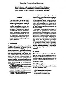
Fig. 1 Key to the diagrams used for displaying the results of the algorithms

method was designed to learn semantics and syntax, but it turns out not to work well on this problem. The HBM works very well; however, it is an active area of research to determine whether such calculations are actually being carried out in the brain. We conclude with a new on-line saturating accumulator developed by the authors, based loosely on the well-known linear reward-penalty algorithm (Yang 2002), and intended to be biologically plausible. Although we are not attempting to measure which algorithm is “best” in any sense, we do need some way to evaluate whether any of them are “successful.” In the interest of consistency, we will display the output of each one using the chart format demonstrated in Fig. 1, with variations appropriate for each algorithm. Each verb is represented by a triangle whose apex is positioned horizontally according to a score indicating its predicted class. Except for some algorithms in the appendix, the score obeys the convention that verbs predicted to be raising should go on the left, verbs predicted to be control go on the right, and verbs predicted to be ambiguous go in the middle. Verbs are evenly spaced vertically using that same inferred order. The filling of each triangle indicates the verb’s known class: shading on the right is raising, no shading is ambiguous, and shading on the left is control. Gray coloring indicates that there are less than 30 occurrences of the verb in the corpus, while black indicates at least 30 occurrences. When appropriate, bars under the triangles indicate how much uncertainty the algorithm has in the placement of the verb, using standard deviation, for example. In all cases, a wider uncertainty bar indicates greater uncertainty. Since some of the algorithms we discuss score the verbs on a continuous interval without predicting discrete labels, decision boundaries for the three classes must be

123


imposed. We adopt the following convention for displaying verbs as being correctly or incorrectly classified: A gray bar is displayed spanning the central third of the gap between used (a raising verb) and the left-most of like and want (control verbs). These verbs were selected because there is plenty of data for them in both the CHILDES and Switchboard corpora. The choice of 1/3 for the width fraction is arbitrary. Ideally, ambiguous verbs lie inside the gray band, raising verbs lie to its left, and control verbs lie to its right. Verbs that lie on the wrong side of one of these decision boundaries are italicized, even if they are in the correct order with respect to the other verbs. Some remarks are in order about what these diagrams are not meant to imply. The output of interest is the predicted classification of each verb as raising, control, or ambiguous. The exact horizontal placements and ordering of the verbs are not of primary interest, rather, such placement yields a representation of how confident each algorithm is in its predictions. Ideally, an algorithm would place all the raising verbs on the extreme left, all the control verbs on the extreme right, and all ambiguous verbs in the middle, with a big gap between each cluster. None of the algorithms achieves this ideal, and the extent to which one of them displaces a raising verb from the left, for example, visually represents its uncertainty about that verb’s classification. Since the algorithms we consider are based on different principles, not all of the horizontal scales are linear, easily comparable, or even in straightforward units. Not all of the algorithms compute error bars, and not every instance of one verb appearing to the left of another is intended to be statistically significant. We considered several additional algorithms that were found to be unsuitable: A perceptron can learn the verb classes accurately, but it requires labeled training data that is not available to children, and it is sensitive to the size of the data set. The field of text mining makes extensive use of matrix-based unsupervised clustering algorithms, but after testing several of these, none was found to work particularly well. In the interest of balancing brevity against the expert reader’s curiosity, we discuss these in the appendix. 4.1 Bayesian Approaches The Bayesian approach to statistics is to use random variables to stand for unknown quantities and for data, then use properties of conditional probability to determine the distribution of the unknowns conditioned on the collected data (Gelman et al. 2004). We specify what are called prior distributions for all of the unknowns when setting up the model. The distributions of the unknowns conditioned on the data are called posterior distributions. Bayes’s formula states that posterior

prior

! "# $ ! "# $ P(model|data) ∝ P(data|model) P(model) .

Bayesian inference is often more successful at analyzing small data sets than traditional frequentist methods. If there is sufficient data, the posterior distribution of an unknown will be concentrated near its underlying value with a small standard deviation. If there is not much data, the posterior will be similar to the prior. It is standard

123


practice to assume uniform or widely distributed priors to minimize the amount of extra information fed to the model. 4.1.1 Bayesian Coin-Flip Model Given the data as in Sect. 3, a reasonable place to start is to compute for each verb the fraction of sentences of each type in which it occurs. To place this on a more solid statistical foundation, we adapt a classic probability problem: Given an unfair coin and a sequence of flip results, estimate the probability that the coin comes up heads. The Bayesian solution is to model the coin by the random variable Q = probability of heads, and assume it has a beta distribution. There is an exact symbolic form for the posterior: Starting with a uniform prior distribution Q ∼ Beta(1, 1) and given m heads and n tails, the posterior distribution is Q|m, n ∼ Beta(1 + m, 1 + n). For large sample size, the posterior is a very narrow peak around the intuitive solution m/(m + n). The mean µ and standard deviation σ of the posterior distribution are √ √ 1+m 1+n 1+m , σ = . µ= √ 2+m+n (2 + m + n) 3 + m + n

Thus, the posterior mean is almost the proportion of heads, with a small modification to allow for the fact that the prior distribution must be valid even with no data. This probabilistic interpretation has the advantage of also generating a measure of uncertainty, the standard deviation, which tends to zero as the amount of data grows. The obvious algorithm is to pick one semantic frame and order verbs by the mean posterior probability that they occur in that frame. The best results are obtained from the animate + eventive frame. Thus, for the jth verb v j , m j is the number of uses of that verb in an animate + eventive frame, and n j is the number of other uses. Then Q j |m j , n j ∼ Beta(1 + m j , 1 + n j ) is the posterior distribution of the fraction of uses of v j in animate + eventive sentences. The verbs are treated independently. This calculation yields the ordering of the verbs by posterior mean shown in Fig. 2. Using the Switchboard data, all of the verbs with at least 30 sentences occur in the correct order except for going and the troublesome have. In the Switchboard data, going is correctly placed to left of need, however, this ordering is not robust: the small change made to the going counts to produce going-st is just enough to move it out of order with respect to need. In the CHILDES data, going occurs out of order with respect to need, as does like. There is a standard frequentist-style statistical test which, given two samples of counts of items with and without a particular characteristic, and a confidence level, states whether there is sufficient data to assert that the two samples are from populations with different proportions of items with the characteristic, and can yield a confidence interval for the difference between those proportions (Devore 1991, Sect. 9.4). Such a test could be applied here to sentence counts for each pair of verbs, but since so many of the verbs occur in very few sentences, the Bayesian approach to confidence is more appropriate here: One can use integrals to calculate the posterior probability that Q for one verb is less than Q for another. A value close to 1 means high certainty and a value close to 1/2 means low certainty. These calculations are shown for some verbs in

123


Fig. 2 Verbs ordered by the mean posterior probability of occurring in an animate + eventive frame using the coin-flip model; Switchboard on the left, CHILDES on the right. Uncertainty bars extend one standard deviation left and right of the mean

Fig. 3 Verb comparisons using the coin-flip model: v1 < v2 indicates that the posterior mean of Q for v1 is less than that for v2 . The ! means the ordering is correct, and × means incorrect. The number indicates the posterior probability P(Q 1 < Q 2 |data). The left table is from the Switchboard data, and the right table is from the CHILDES data

Fig. 3. Most of the correct comparisons come with high confidence, but in the Switchboard data, want and have are very robustly misplaced, and the placement going-st with respect to need and want is uncertain. In the CHILDES data, the incorrect ordering of like and need is quite robust. Thus, ordering by proportions works reasonably well, but fails to correctly and robustly place going and makes other mistakes. In search of better results, we discuss two more sophisticated Bayesian models.

123


4.1.2 Bayesian Approach Based on A&S Alishahi and Stevenson (2005a,b, 2008), which we will abbreviate A&S, likewise focus on the learning of verb-argument structure, although they have a somewhat different goal from our work. They adopt a Bayesian framework to model the phenomenon of children’s overgeneralization errors using intransitive verbs in a transitive frame with a causative meaning (causative meaning is compatible with a transitive syntactic frame but not typically with an intransitive syntactic frame). For example, children sometimes say “Adam fall toy” to mean Adam makes the toy fall (Bowerman 1982). In A&S’s model, similar syntactic frames (e.g., transitive, intransitive, ditransitive, etc.) are grouped together according to their shared semantic properties, where semantic properties are understood as (combinations of) primitive features such as cause or move. Syntactic frames, which include the verb, are associated with semantic properties with a certain probability. The more frequently a given semantic feature appears in general, the higher its probability of being associated with a given individual syntactic frame. A&S show that after running their learning simulation on 800 input utterance-meaning pairs using the most common verbs found in the mothers’ speech in the Brown (1973) corpus, their learner managed to learn these verbs with the expected U-shaped learning curve. Moreover, the learner made some of the same overgeneralizations in sentence frame use in the production portion of the test that actual children make (e.g. inserting an intransitive verb in a transitive frame with causative meaning). Crucially, A&S assume that the learner is able to deduce both the syntactic frame of the sentence they are perceiving, and also the meaning of the utterance based upon perception of the nonlinguistic scene that is co-occurring with the utterance. The problem we are interested in is significantly more difficult than the one tackled by A&S (and, therefore, these assumptions do not hold), for two reasons. One is that syntactic ambiguity is involved in parsing the string, such that we do not assume that the learner can immediately deduce the structure upon hearing the string. Secondly, given the abstractness of the verb meanings we are interested in, we do not assume that the child can immediately determine the meanings of these verbs based on observation of the environment.6 In fact, as A&S correctly point out, the syntactic frame of a verb and its lexical meaning are closely tied together, such that if children could immediately determine the meaning of want or seem upon hearing it in a sentence and observing a scene, knowledge of the syntactic properties of the sentence would follow. But for the reasons just cited neither the full structure of the sentence nor the meanings of abstract verbs are available a priori to learners for the types of sentences we are interested in. Although the algorithm described in A&S is not immediately applicable to our problem, it can be adapted as follows. Identifiers in CodeStyle text refer to specific components of the computer program that implements the calculation. The algorithm iteratively adds sentences from an input sequence to a complex data structure built of Sentences, Frames, Constructions, and LexicalEntries.

6 The idea that children could deduce the meaning of any verb, even concrete ones, based on observation

of the world is challenged in the syntactic bootstrapping literature; see Gleitman (1990).

123


Each Sentence consists of a String naming its main verb and a Frame representing its basic semantic content. Each Frame has two Features, a subject animacy that is either True or False, and a predicate eventivity that is either True or False. In contrast to A&S, no other syntactic information is associated with a sentence because all the sentences of interest have the same surface form (subject, verb, infinitival predicate), and we are interested in deducing the appropriate hidden syntax. If the learner already knew for example whether the verb requires, allows, or forbids a semantic subject, then this acquisition problem would have already been solved. A Construction is a mapping from Frames to counts of how many times each Frame has been added to the Construction. A LexicalEntry contains a String naming its verb and a mapping from Constructions to counts of how many times each Construction has been linked to that LexicalEntry. For each Sentence in the list of input, the algorithm adds it to one Construction, within which the count for that Sentence’s Frame is incremented. The choice of which Construction the new Sentence should be attached to is as follows. We hypothesize that the prior probability of choosing Construction k is P(k) =

nk N +1

(18)

where n k is the number of Sentences attached to k, and N is the total number of Sentences seen so far. A bit of mass is reserved in this prior for the case that a new Construction, denoted ∅, is needed, P(∅) =

1 N +1

(19)

The probability of Feature i of a random frame f given Construction k is P( f i |k) =

(count of Frames in k with Feature i = f i ) + λ n k + λαi

(20)

where i is Subject or Predicate. The intuition of this formula is that to sample a Feature given a Construction, one picks a Frame from it uniformly at random, and reads Feature i from that Frame. However, some accommodation must be made for new Constructions, which have no Frames yet (n k = 0). So we add small numbers to the numerator and denominator, which avoids division by 0 when n k = 0 and leaves room to specify that the distribution of Feature i of a random Frame f given an empty Construction is P( f i |∅) =

1 αi

(21)

The value of αi is the number of possible values that Feature i can take. In other words, if no other information is available, assume each Feature value is equally

123


% likely. The constant λ should satisfy 0 < λ < i 1/αi for reasons explained in Alishahi and Stevenson (2008). Since both the subject and predicate can take on two values in this problem, αSubject and αPredicate are both 2, and λ is no more than 41 . The probability of a Frame f given Construction k is the product of the probability of its Features given k, P( f |k) = P( f Subject |k)P( f Predicate |k).

(22)

This formula holds assuming that the Features are independent, as in A&S. The probability of a Construction k given a Frame f may now be computed with Bayes’s formula, P(k| f ) ∝ P(k)P( f |k).

(23)

When a new Sentence arrives consisting of a verb v and a Frame f , it is added to the Construction k such that P(k| f ) is maximum, including the possibility of a new, empty Construction. The count on the link from the LexicalEntry for v to k is then incremented. The expectation is that the algorithm will discover Constructions representing raising verbs and control verbs, and counts on the links will indicate which verbs belong to which class. The algorithm was fed a sequence of random sentences distributed according to the proportions found in the Switchboard corpus. The outcome is very consistent: It creates four Constructions, each of which contains exactly one of the four possible Frames, and the counts for how many times each verb is linked to one of these four Constructions is just number of times it appears in that one Frame. So despite the probabilistic framework, the algorithm ends up essentially reproducing Tables 4, 5, and 6. If the parameters αSubject , αPredicate , and λ are made larger than what is specified in A&S, it is possible to get the algorithm to make Constructions that contain all animate or all inanimate Frames discarding predicate eventivity, but even less information about the verbs can be derived from this output. In summary, even though the algorithm in A&S seems to be designed for exactly this kind of problem, it turns out not to work at all. 4.1.3 Hierarchical Bayesian Inference The method of Perfors et al. (2010), Kemp et al. (2007), which makes use of a hierarchical Bayesian model (HBM), can be adapted to the problem of distinguishing raising and control verbs. Perfors et al. (2010) apply it to the problem of learning which verbs taking two objects can be used in double object dative constructions (as in John gave Fred a book) and which ones require a preposition on the second object (as in John donated a book to the library). Using data from corpora similar to ours, they infer the usage rates of several verbs in each of these constructions, and simultaneously infer the learner’s underlying assumptions. The raising-control distinction is different in that the surface strings for both underlying syntactic trees are the same, so we will

123


instead infer how strongly a verb prefers an animate syntactic subject, assuming that verbs with a very strong preference use control syntax. For the raising and control problem, the setup is as follows, based on Model L3 of Perfors et al. (2010). For each verb v, the unknown proportion of sentences in general speech in which it is used with an animate subject is Av . The number of animate subjects in a sample of n v sentences with that verb is therefore a random number with the binomial distribution with parameters Av and n v . We assume that Av lies somewhere on a scale between very selective (Av = 1) and flexible (Av ≈ 0.5). We represent that selectivity with a number λv between 0, meaning completely flexible, and 1, meaning highly selective. Since each λv is an unknown number between 0 and 1, we give them a beta distribution with parameters γ1 and γ2 as priors. We hypothesize that flexible verbs occur with animate subjects at unknown rate β. For each verb Av = λv + (1 − λv )β. Since β is an unknown number between 0 and 1, we assume that it has a beta distribution, with parameters φ1 and φ2 . The hyperparameters γ1 , γ2 , φ1 , and φ2 are also unknown but are probably not large, so for their prior, we model them as coming from an exponential distribution with parameter 1. Given such a probability model, Bayes’s formula can estimate the distribution of the unknowns conditioned on data. For each corpus, the complete set of data counts for all verbs is analyzed together. The posteriors of the various unknowns have no exact symbolic solution. Instead, determining the posterior distribution requires using a Markov Chain Monte Carlo (MCMC) method to approximately integrate over the unknown parameters. Mitchener used a program called JAGS, available from http://mcmc-jags.sourceforge.net, to perform the calculation. The JAGS computation yields an approximate posterior density for each λv , indicating the probability that λv takes on each possible value between 0 and 1, conditioned on the data. Sorting verbs by λv should group them into the three classes. Figure 4 displays the verbs in order of the means of these posterior densities. As in Sect. 4.1.1, one can estimate the posterior probability that λv1 < λv2 by counting how many times a sample of λv1 is less than a sample of λv2 , and computing the fraction of such comparisons out of the total number of comparisons. These estimates are shown in Fig. 5. For the Switchboard data, the model is very confident that the control verbs are highly selective. Except for begin and start, for which there is less data, all the verbs are ordered correctly. Even the troublesome have is correctly placed. However, there is much more uncertainty with most of the raising verbs. The margin between have and try is very slim. For the CHILDES data, the order of going, need, and used is scrambled and uncertain. The verbs love and begin are also distinctly out of place, but this is a less serious problem because there is little data for those verbs. The advantage of having a hierarchy of unknowns is that the inference process can estimate assumptions that lie several layers under the data [called overhypotheses in Perfors et al. (2010), Kemp et al. (2007) and hyperparameters in Gelman et al. (2004)]. For both corpora, the values of γ1 and γ2 are determined with high confidence (standard deviation on the order of 10−17 ). These determine the distribution of a typical

123


seem begin start tend happen going

begin

going st

love

used

seem eq

continue

seem

need

used have

need

try

0.0

0.2

0.4

0.6

going

want

want

choose

hate

hate

like

like

start

love

try

0.8

1.0

0.0

0.2

0.4

0.6

0.8

1.0

Fig. 4 Results of running hierarchical Bayesian inference for verb selectivity for animate subjects; Switchboard on the left, CHILDES on the right. Each verb v is centered at the posterior mean of λv . Uncertainty bars extend one standard deviation left and right of the mean Fig. 5 Verb comparisons: v1 < v2 indicates that the posterior mean of λv1 is less than that of λv2 . The ! means the ordering is correct, and × means incorrect. The number indicates the posterior probability P(λv1 < λv2 |data). The left table is from the Switchboard data, and the right table is from the CHILDES data

λv when the verb is unknown (see Fig. 6). The peaks at the endpoints are consistent with the intuition that verbs are typically either selective or flexible. The posterior distribution of β, shown in Fig. 7, is determined by φ1 and φ2 , which are much more uncertain (standard deviations of 0.9). Since β’s distribution is so spread out, the data

123

W. G. Mitchener, M. Becker Fig. 6 Posterior density for λv : a beta distribution using the parameters γ1 = 0.521858 and γ2 = 0.14353, means of the posteriors inferred from the Switchboard data

2.0

1.5

1.0

0.5

0.0

Fig. 7 Posterior density for β: a beta distribution using the parameters φ1 = 0.956321 and φ2 = 1.30087, means of the posteriors inferred from the Switchboard data

0.2

0.4

0.6

0.8

1.0

0.2

0.4

0.6

0.8

1.0

2.0

1.5

1.0

0.5

0.0

suggests that there is no typical value of β for a random flexible verb, that is, flexible verbs occur with animate subjects at a wide variety of rates. It is possible to perform the same calculation on each verb’s selectivity for eventive predicates, but the results are not as good. The Switchboard data yields a mostly correct ordering of the verbs, but with a very narrow range of λ. The CHILDES data yields a rather scrambled ordering of the verbs. Overall, this model gives very good results on the Switchboard data, but not as good results on the CHILDES data. Furthermore, even on the Switchboard data, the margin between control verbs and ambiguous verbs is very slim. The MCMC calculation performed here by JAGS is appropriate for a digital computer, but it is unlikely that neural networks use this algorithm. However, there are other ways of implementing the same Bayesian calculation. For example, one could represent posterior densities directly, perhaps as polynomial splines or spike rates, and update them as each new data point arrives. Recent studies have found evidence that neurons can encode probabilities in their spike patterns, and that their natural integration ability might be performing Bayesian calculations (Deneve 2008a,b). So it appears that HBMs such as this one might indeed be implemented more or less directly by the brain, but this is an area of active research.

123


4.2 Saturating Accumulator 4.2.1 Motivation In a final attempt to demonstrate that this verb classification problem can be solved using simple calculations that are neurologically plausible, we now formulate a new online accumulator algorithm based on reformulating and improving the linear rewardpenalty learning model. Consider a learning device receiving a sequence of sample sentences using a particular verb in one of the four semantic frames. It needs to have a state that can settle into equilibria representing the extremes of purely raising and purely control, but also into intermediate equilibria for ambiguous verbs. The state should change with a balance of skepticism and the ability to saturate. Skepticism means that if an isolated sample sentence comes along that contradicts the current state of the register, then it might be noise and should be ignored. Saturation means that when a sample sentence comes along that reinforces the current state of the register, then the state should remain nearly the same. However, if several sample sentences are given that contradict the current state, then it should change. Such a device might be implemented by a small neural network in which the state is represented by how many of a handful of excitatory neurons are connected to an output neuron. The widely-studied linear-reward-penalty (LRP) algorithm (Yang 2002) has several of these properties. The algorithm maintains a value x between 0 and 1, and changes x in response to a sequence of signals that it should move left or right. For a move to the left, the new value is ax, and for a move to the right, the new value is ax + (1 − a), where a is a positive constant that controls the step size. Given a substantial amount of data in one of the directions, LRP approaches saturation: When x is close to 0 or 1, further steps in that direction do not change its state significantly; that is, LRP ignores surplus data that merely reinforces its current knowledge. Unfortunately, it takes the biggest step to the left when its state is close to 1 and it takes the biggest step to the right when its state is close to 0. Thus, it fluctuates strongly in the presence of noise. Although it can converge to 0 or 1, it has no intermediate stable equilibrium. This property makes it unsuitable for representing ambiguous verbs, which neither require nor forbid a semantic subject and lie in a gray area. One variant, LRPB (linear-reward-penalty-batch), adds a batch counter so that the algorithm takes a step only when several items indicating one direction have been processed (Yang 2002). LRPB is skeptical about taking steps in directions inconsistent with the information it has seen so far. We sought but were not able to find parameters for LRP or LRPB that could accept a sequence of frames and reliably indicate that the verb preferred, accepted, or dispreferred that frame. We developed a new saturating accumulator algorithm as a way to adapt LRP so as to have the skepticism of LRPB and have intermediate equilibrium states suitable for representing ambiguous verbs. The saturating accumulator algorithm is also designed to mimic the gradual learning process observed by Becker (2006). When learning a verb, the initial state of the particles is neutral, allowing all types of sentences, and only with a significant amount of data do some types become strongly preferred or dispreferred. This parallels the tendency of young children to accept control verbs in syntactic contexts that are

123


appropriate only for raising syntax, and gradually learn the proper usage as they acquire the adult grammar. 4.2.2 Mathematical Details Each verb is represented by a system of four particles, one for each semantic frame. Each particle is located between −1 and 1, and the overall system is represented by a position vector x(t) = (xAE (t), xAS (t), xIE (t), xIS (t)). A positive value of one of the x variables indicates a preference for the corresponding frame, and a negative number indicates an aversion. A particle at location x experiences a force due to an ambient field with potential v(x) = − cos(5π x). The overall potential on the particle system is V (x) = v(xAE ) + v(xAS ) + v(xIE ) + v(xIS ).

(24)

The force on the particle system due to the force field at time t is the vector Ffield = − grad V (x(t)) For each particle, the potential has 5 wells between −1 and 1. To encourage the particles to settle down at the bottom of one of these wells, we add friction terms. Each particle experiences a damping force proportional to its velocity. In vector notation, these forces are of the form Ffriction = −β

dx dt

where the constant β is a parameter to be determined. Each sample sentence exerts a force as follows. Each semantic frame is associated with a particular pattern vector: ' & 1 1 1 pAE = 1, − , − , − 4 4 2 ' & 1 1 1 pAS = − , 1, − , − 4 2 4 ' & 1 1 1 pIE = − , − , 1, − 4 2 4 ' & 1 1 1 pIS = − , − , − , 1 2 4 4

(25)

The pattern pAE for animate eventive sentences comes from setting the AE entry (first entry) to 1, setting the entries for frames that differ in one aspect (IE and AS) to −1/4, and setting the entry for the frame that differs in both aspects (IS) to −1/2. The total of the pattern is 0. The AE particle is given a push toward 1, and the other particles are given a push toward −1. The other three pattern vectors are constructed similarly.

123


When a sentence with frame f arrives at time t0 , it creates a force on the particles with potential L(x, t, f, t0 ) =

(

0 1 −(t−t0 )/σ 2e

if t < t0 , ) ) )x − p f )2 if t ≥ t0 .

(26)

This sentence’s contribution to the potential pushes the particle system toward the pattern p f . The exponential part causes the force to weaken over time as controlled by a decay parameter σ . The force at time t generated by sentence i with frame f i arriving at time ti is given by Finput = −γ grad L(x(t), t, f i , ti ) where the gradient is taken with respect to the entries of x and the constant γ is a parameter to be determined. The overall behavior of the particles is governed by the differential equation * d2 x(t) = F + Finput + Ffriction field dt 2 inputs + , * dx(t) = − grad V (x(t)) − γ grad L(x(t), t, f i , ti ) − β dt

(27)

i

The constants γ and β control the relative magnitudes of the forces from input sentences and friction. The sum is over all inputs, where the ith input is a sentence with frame f i that arrives at time ti . 4.2.3 Results and Interpretation The accumulator includes three parameters, σ , γ , and β. In addition, the rate of arrival of input sentences is unknown. However, some trial and error shows that if sample sentence ti arrives at t = i (a rate of one input per time unit), then the following parameter values give reasonable results: σ = 10, γ = 8, β = 8

(28)

With these values, the differential equation (27) may be solved by standard numerical methods. As a first test of the algorithm, we pick a verb and feed 100 randomly created sentences to the algorithm. The semantic frames are generated in proportions matching that verb’s occurrence with animate/inanimate subjects and with eventive/stative predicates in the CHILDES data. The particle dynamics run out to time t = 110 to give the system 10 time units to settle after the last input arrives. See Figs. 8, 9 and 10 for time traces of the particle positions for each verb. For each of these pictures, the particle positions xAE (t), xAS (t), xIE (t), and xIS (t) are plotted as functions of time t.

123


AE

AS

IE

IS

Fig. 8 Particle dynamics tests for used using proportions matching the CHILDES corpus

AE

AS

IE

IS

Fig. 9 Particle dynamics tests for need using proportions matching the CHILDES corpus

AE

AS

IE

IS

Fig. 10 Particle dynamics tests for want using proportions matching the CHILDES corpus

The horizontal scale for each trace represents time flowing from 0 to 110. The vertical scale for each trace is −1 to 1. Next to each trace, the final location of each particle is shown superimposed on the ambient potential v(x), with x running from −1 on the left to 1 on the right. The potential diagrams correspond to the right-most points of the time traces rotated a quarter turn. At the end of the learning process, each particle settles into one of five wells in the ambient potential. We discretize each particle’s final state to a row of five squares, one for each well, where the square corresponding to its rest position is colored black. The four rows are stacked to give the pattern displayed to the right of each verb’s time traces. The control verb want shows a very strong preference for animate + eventive in that xAE remains very high, along with an aversion to inanimate subjects in that xIE and xIS

123


Fig. 11 The three most frequently occurring patterns (labeled A, B, and C) and the percentage of trial runs in which they occur

remain low. The ambiguous verb need shows an intermediate pattern with some preference for animate + eventive, but less aversion to inanimate + eventive. The raising verb used shows an even weaker preference for animate + eventive. The extent to which the accumulator can distinguish the classes is made clearest by running the algorithm many times on different sets of randomly generated sentences for each verb, and building a histogram of its final states. There are three final states (labeled A, B, and C) that occur many times when learning the verbs try, want, need, and going, as shown in Fig. 11. For each combination of corpus and verb, these patterns occur at characteristic frequencies. The strongly raising verbs seem and tend do not exhibit these patterns. This observation suggests that the fraction of runs of the algorithm that end in one of these three patterns might make a suitable index for classifying verbs. A vector counting occurrences of these patterns could conceivably be used in place of the scaling procedure used in clustering algorithms, as it accomplishes essentially the same thing (see Appendix): It compensates for the fact that some of the verbs are very common, and certain uses of certain verbs obscure the fact that they can be used in other ways. It turns out that there is no need to invoke a complex clustering algorithm on the pattern counts. We define the following index, H = A + B + max{A, B, C}

(29)

where A is the percentage of times the verb causes the algorithm to end up in pattern A, and likewise for B and C. The A + B term is included because it is large for control verbs. The maximum of A, B, and C is included because it is rather low for going and other control verbs: They can be used in a greater variety of patterns which leads to a greater variety of final states. The result of ordering most of the verbs listed in Sect. 3 by H is shown in Fig. 12. For the Switchboard data, most of the verbs occur in the correct order. The exceptions are have, and three verbs that are rare in the corpus, continue, start, and begin. For the CHILDES data, going and like occur out of order, but the other common verbs are ordered correctly. 5 Discussion and Conclusion We began with the broad question of how language learners determine the underlying structure of a string, given that even with knowledge of basic word order of a language,

123

W. G. Mitchener, M. Becker begin seem happen tend start used

seem

going

seem eq

going st

used

need

love want

like

hate

going try

need

continue

want

have

begin

like

hate

choose

start try

love 0

50

100

150

200

0

50

100

150

200

Fig. 12 Verbs sorted by the index H ; Switchboard on the left, CHILDES on the right

many sentence strings are potentially compatible with multiple underlying structures. Our approach relies on the tight coupling of verb category (as categorized in terms of verbs’ argument-taking properties) and the syntactic structures a verb participates in, so that categorizing a verb correctly will lead to understanding the syntactic structure of otherwise ambiguous strings. Focusing on the case of a string that could host either a raising or a control verb in the matrix verb position (and the category of the matrix verb determines the structure of the sentence), we argued that the learner cannot simply resolve the ambiguity of this string with a subset-type strategy. That is, the learner cannot assume that a novel verb in this string is a control verb, on the supposition that an incorrect assumption will be defeated by hearing the verb with an expletive subject. The key reason is that the class of ambiguous verbs (begin, start, need, etc.) occur in all of the sentential environments that both raising and control verbs do. Thus, there is no proper subset relation between the constructions raising and control verbs occur in. Although evidence of a verb’s occurrence with expletive subjects provides useful information to learners (and learners are certainly expected to use this information), we have argued that learners additionally rely on semantic cues within the ambiguous string in a probabilistic manner, in order to distinguish the classes of raising, control and ambiguous verbs. Based on experimental evidence from adult speakers, we identified two relevant basic semantic features: animate vs. inanimate subjects, and eventive vs. stative embedded predicates. The simple classification strategy of looking at the proportions of a verb’s use in the four semantic frames fails. Usage rates give an elementary means of classifying verbs, however, there are no thresholds on the proportions that correctly and robustly

123


classify all the data from the corpora. Some verbs are used overwhelmingly with animate subjects and eventive predicates, and these drown out the fact that the verb can be used in distinctly raising contexts. A&S’s Bayesian approach was developed specifically for learning how semantics maps to syntax, and it can be adapted for classifying raising and control verbs. However, it turns out not to work at all, and reproduces the counts of frames present in the data. A hierarchical Bayesian model, based on Perfors et al. (2010), Kemp et al. (2007) yielded good though possibly fragile results on the Switchboard data, but had trouble with the CHILDES data. Overall, this algorithm produced the most promising results from potentially biologically realistic calculations. We also developed an on-line saturating accumulator algorithm, based on LRP and intended to be biologically realistic. Tests of this algorithm reveal that it is capable of distinguishing different classes of verbs from the frequencies of their use in basic semantic frames. An index based on the fraction of runs of the algorithm that end in each of three states sorts verbs from control to raising that correctly orders the most common such verbs (except for have) in the CHILDES and Switchboard corpora. However, the thresholds between verb classes are clearly different between the two corpora. Other disadvantages of this algorithm are that it is complex, and the selection of parameters is somewhat ad-hoc. Furthermore, it is quite different from the well-studied algorithms of statistical learning theory, and further study is required. The overall results are summarized in Table 7. Again, the purpose of this project is not to choose a “best” algorithm, but to determine if certain information is present in the primary linguistic data. These algorithms all produce some ordering of the verbs, and marks in this table indicate whether each one correctly orders a test verb with respect to several reference verbs when given data from just one corpus. These criteria were selected for display based on the discussion at the beginning of Sect. 4. The summary table shows that several of the algorithms tested were able to mostly classify, cluster, or sort those verbs that are well-represented in the CHILDES and Switchboard data. This supports the possibility that the primary linguistic data contains statistical patterns that provide implicit negative evidence, thereby enabling children to deduce over time that certain verbs cannot be used in certain semantic and syntactic constructions. Each of the algorithms had at least some difficulty with the task, which suggests that subject animacy and predicate eventivity alone provide insufficient data for correctly learning all aspects of these verbs. However, such information suffices to give young learners a good start toward deducing the full meanings of these verbs, which is known to take up to age five or later (Becker 2006). Importantly, we assume that the learner makes certain assumptions about language structure prior to experience. For instance, the learner must assume that similar strings can be associated with divergent underlying structures, and that semantic relationships need not be local (i.e., the subject of the sentence might be semantically related only to a predicate in a lower clause, not the immediately string-adjacent verb). In addition, to derive the semantic properties of these verbs, learners must be biased to assume that inanimate or expletive subjects are unlikely to be agents (along the lines of Dowty (1991) or Keenan (1976)), and therefore that verbs that occur with these subjects are unlikely to assign them a thematic role. These assumptions are necessitated by the

123

123

Proportions SB

!

!

!

×

!

!

!

!

×

!

!

!

!

!

!

!

!

!

!

!

!

!

!

!

Like

×

!

×

Want

!

!

×

!

×

!

Need

Going

×

!

!

!

×

!

Like

!

!

!

!

!

!

Want

!

!

×

Need

Going-st

!

!

!

Like

The corpus tested in each row is indicated at the left, SB for Switchboard, CH for CHILDES. CHILDES does not include have or going-st so those spaces are blank

CH

Sat. accum. SB

CH

HBM SB

CH

Used

Like

Used

Want

Have

Need

!

!

!

Want

Table 7 Summary of algorithm performance: ! means the test verb (very top) is correctly ordered with respect to the reference verb (underneath) and × means they are inverted



particular learning problem at hand: the classes of raising, control and ambiguous verbs could not be distinguished without these assumptions (for instance, on a purely input-based learning model). However, if these assumptions are in place for learning this particular set of verb classes, they should in principle be available for learning other classes of verbs. We hold the view, then, that learners bring these assumptions about language to bear on the language learning task in general. All of the algorithms discussed here exhibit divergence between the Switchboard and CHILDES data: The thresholds between the different classes of verbs are unequal.7 There is therefore evidence that either these particular corpora are unrepresentative of actual speech, or more likely, that child-directed speech uses generally different proportions of animate and eventive predicates than adult-directed speech. Such sentence strings could be associated with either raising or control syntax and in that sense offer less information than the other three semantic frames. If children are discarding such sentences as uninformative, then the bias in child-directed speech in favor of them might contribute to the tendency of young children to accept control verbs in raising constructions: Initially, the child-directed speech they hear contains insufficient information and they misclassify many verbs. As they age, they hear more adult conversation, which contains more informative sentence types and should eventually lead them to learn the proper class for each verb. In future work, the statistical differences between adult and child directed speech should be studied, including the extent to which patterns observed in child language acquisition may be attributed to these differences versus features of the underlying learning algorithm. Acknowledgments This material is based upon work supported in part by the National Science Foundation (grant #0734783) (Mitchener) and a Junior Faculty Development grant from UNC (Becker). The authors would like to thank Lisa Pearl, William Sakas, Charles Yang, the audience and participants at the Workshop on Psychocomputational Models of Human Language Acquisition 2007, and two anonymous referees for their many useful suggestions. We also thank Susannah Kirby, Louise Lam and Seema Patidar for coding assistance.

A Some Additional Algorithms In this appendix, we discuss some additional algorithms that were either clearly less successful than the ones in the main text, or had a theoretical flaw. We present them here as further evidence that the basic semantic information we consider is sufficient to at least begin separating the verbs of interest into the three classes, and that this classification problem is non-trivial. A. 1 Perceptron The perceptron is a simple learning algorithm that is a reasonable starting point for small classification tasks. It is trained on examples consisting of vectors of numbers, each labeled to indicate its class. Once trained, it predicts the label for an input vector by the sign of a linear combination of the vector’s elements. We do not consider it in 7 Also, a perceptron trained on one corpus does not work well on the other; see the Appendix.

123


the main body of the paper because the labeled training data it requires is not available to children. However, it turns out to be successful at the learning task, so we include it here. A basic perceptron can only distinguish between two classes, so we use a double perceptron to deal with the three verb classes of interest. Each verb will be classified as either +raising or −raising and either +control or −control. A control verb should be labeled −raising and +control. A raising verb should be labeled +raising and −control. An ambiguous verb should be labeled +raising and +control. None of the verbs in this study should be labeled −raising and −control. The input consists of vectors of counts of how many times each verb appears in each semantic frame {AE, AS, IE, IS} in each corpus. For each verb v, let nv be its count vector, nv = (n v,AE , n v,AS , n v,IE , n v,IS ), let yv,R be 1 if the verb is raising or ambiguous and −1 if not, and let yv,C be 1 if the verb is control or ambiguous and −1 if not. The training process finds weights λt, f for each semantic frame f ∈{AE, AS, IE, IS} and each feature t ∈ {R, C}, and biases βt for each feature. The perceptron consists of the resulting classifier functions PR (n) = n · λR + βR PC (n) = n · λC + βC which predict whether the verb with counts n can be used with each kind of syntax. The sign of PR (n) should be the correct label ±raising for the verb, and the sign of PC (n) should be the correct label ±control. The magnitudes of PR and PC indicate confidence of the label. Specifically, they are proportional to the geometric distance from the count vector to a hyperplane separating the + and − classes for each feature. The weights and biases are chosen to minimize S=

*

v∈T

. . exp −yv,R PR (nv ) + exp −yv,C PC (nv )

(30)

/ / subject to the constraint that f λR, f = f λC, f = 1, where T is a training set of verbs. The perceptron was first trained on the Switchboard data, and it correctly labels all the training data. Results are shown in Figs. 13 and 14. The horizontal position of each verb in the left-hand pictures is PR (n), which indicates how certain the perceptron is that each verb is +raising, and similarly for +control in the right-hand pictures. Most of the verbs are placed relatively close to the decision boundary, so a second picture with a stretched horizontal scale shows those verbs more clearly. Although this perceptron correctly labels the training data, it mislabels most of the CHILDES data, specifically used, need, going, start, and begin. The problem seems to be variation in the overall sample size of each verb. For the verb going, the sample size is much larger in CHILDES than in Switchboard. In contrast, the sample size for other verbs is smaller in CHILDES than in Switchboard. It is therefore not surprising

123

Computational Models of Learning the Raising-Control Distinction seem

seem

used

tend

happen

start

going

going

tend

going st

going st

have

start

need

need

begin

begin

happen

choose

used

continue

continue

love

try

hate

want

try

choose

like

love

have

hate

want

like 0

50

100

150

10 000

going

5000

0

5000

happen

going st

going

have

tend

need

going st

begin happen

start

used

need

continue try

begin

want

choose

choose

continue

love

love

hate

hate

like 20

10

0

10

20

600

400

200

0

200

400

Fig. 13 Results of training and running the perceptron on the Switchboard data to classify verbs as ±raising on the left, ±control on the right. Horizontal placement of verb v is by PR (nv ) on the left and PC (nv ) on the right. The lower pictures show the same data with zoomed horizontal axes. The vertical reference line is at 0. In each picture, verbs to the right of 0 are labeled +feature

that this classifier has trouble with the CHILDES data. The linear perceptron has the property that nonzero bias terms βR and βC introduce dependence on the sample size. For example, when this perceptron is tested on data formed by tripling all the counts from the same Switchboard data it was trained on, it mislabels try, need, start, and begin. Training the perceptron on the CHILDES data yields similarly mixed results, as shown in Fig. 14. The resulting perceptron correctly classifies all the CHILDES verbs on which it was trained except for mislabeling start and begin as −raising. Importantly,

123

W. G. Mitchener, M. Becker seem eq

seem eq

seem

used seem

need going

going

used

love

hate

like

begin

begin

start

hate

love

need

try

start try

like want

want 10

5

0

5

10

300

200

100

0

100

200

300

Fig. 14 Results of training and running the perceptron on the CHILDES data: ±raising on the left, and ±control on the right. Horizontal placement of verb v is by PR (nv ) on the left and PC (nv ) on the right. The vertical reference line is at 0. In each picture, verbs to the right of 0 are labeled +feature

it correctly labels the troublesome going. However, when tested on the Switchboard data, it mislabels going and used as +control, and need, begin, and start as −raising. A. 2 Spectral Clustering Spectral clustering is a family of techniques that use singular value decomposition (SVD), also known as principal component analysis (PCA), to split the columns of a matrix into sets of similar items. The singular values of a matrix are related to the spectrum of a linear operator, hence the name. Spectral clustering and related algorithms are well known in the data mining and computational linguistics communities. In Boley (1998), columns are interpreted as documents, rows are interpreted as terms, entries of the matrix are counts of how often each term appears in each document, and the goal is to cluster the documents. Adapting Boley (1998) to the problem of clustering verbs, consider a matrix K with one column for each verb and one row for each semantic frame, where the (i, j)th entry is the number of times verb j occurs in frame i. A scaling procedure is applied to each column of K so that its Euclidean norm is 1, yielding a matrix M. The centroid w is defined as the average of columns of M, and the matrix A is defined by subtracting w from each column of M. The intuition behind these transformations is that K represents verbs directly as points in four dimensional space, M is their projection onto a unit sphere, and A is the result of re-centering the cloud of points to the origin. The scaling procedure is a way of compensating for the fact that some verbs are more common in the corpus than others, but is geometrically different from using usage frequencies derived by dividing each column by its sum. The next step is to apply the SVD to the matrix A, which determines matrices U, V, and W such that A = UWVT , U and V are orthogonal matrices, and W is a diagonal matrix (whose diagonal entries are in decreasing order) with additional columns of zeros. This decomposition constructs rotated coordinate axes (the columns of U) that

123


match the ovoid structure of the point cloud A. The first column of U picks out the principal direction, in which the point cloud is widest. The matrix V gives new coordinates for each point with respect to these rotated axes. The meaning of a unit length in these coordinates depends on the magnitudes of entries of K and the scaling function. Clusters are formed by looking at the first column of V, and using 0 or some other threshold to divide the point cloud into left and right sub-clouds. Those can then be further subdivided by recursively applying the algorithm, or by using other columns of V. Clustering algorithms generally require some tweaking to get the best results. In this case, given all the Switchboard data, spectral clustering partially separates the verbs with fewer sentences, apparently ignoring their preferences for the different semantic frames. This disturbs the separation of the other verbs. Better results are obtained when the data contains only verbs with at least 30 occurrences. Furthermore, seem is widely separated from the other verbs, so it makes sense to place it in a cluster by itself and recursively cluster the remaining verbs. Applying this calculation yields Fig. 15. The raising and control verbs are distributed along the principal direction with control verbs preferring one end and raising verbs preferring the other. Neither corpus yields a completely correct ordering, and no threshold perfectly separates the three classes. The CHILDES data yields an essentially scrambled order. Oddly, when seem is included with the Switchboard data, the raising verb tend is placed at the far right, which is completely wrong. There are a variety of other spectral clustering methods. The main differences are in the scaling procedure and in the process for further subdividing the clusters. The different scaling procedures are attempts to compensate for the fact that some documents are longer than others, or in the language of the current problem, that some verbs are more common than others. Finding the best scaling for a particular problem is largely a matter of trial and error. To give an example of another scaling procedure, Boley (1998) mentions a more complex one called TFIDF, however, this scaling gives equally disappointing results on this problem. Thus, although spectral clustering partially separates the verbs, it is not able to identify the three classes particularly well.

A. 3 Non-negative Matrix Factorization and Clustering Non-negative matrix factorization (NMF) is a family of techniques developed to decompose collections of vectors representing objects into linear combinations of features in such a way that the features have all entries zero or positive, and coordinates of the original vectors with respect to the features are all zero or positive (Lee and Seung 1999; Berry et al. 2007; Paatero and Tapper 1994). NMF also allows for soft clustering, in which the new coordinates of an item from a collection can be interpreted as the confidence with which that item can be assigned to each cluster. Unlike SVD, there is no unique or canonical NMF. Some NMF algorithms are based on random numbers and may therefore yield different results on every run. Many that work well in practice are not well understood theoretically.

123

W. G. Mitchener, M. Becker happen tend used want need

used

going

like

going st

want

have

going

like

need try

0.6

0.4

0.2

0.0

try

0.2

0.6

0.4

0.2

0.0

0.2

0.4

Fig. 15 Results of spectral clustering with unit scaling, excluding seem and verbs with fewer than 30 occurrences; Switchboard on the left, CHILDES on the right. Verbs are placed according to the first column of V, their coordinate in the principle direction happen tend used going going st

used

need

like have

want want

going like

need try

0.0

0.2

0.4

0.6

0.8

try

1.0

0.0

0.2

0.4

0.6

0.8

1.0

Fig. 16 Results of NMF clustering, excluding seem and verbs with fewer than 30 occurrences; Switchboard on the left, CHILDES on the right. Verbs are placed based on their scaled attachment strength wˆ i, j to the most correct cluster j

Of the many NMF algorithms under active research in the data mining community, we will focus on one called alternating least squares (ALS), which takes an m × n matrix A and a rank k, and attempts to find an m × k matrix W and a k × n matrix H, both with all entries non-negative, such that the Frobenius norm of A − WH is minimized. The Frobenius norm of a matrix is the square root of the sum of squares of its entries. The algorithm proceeds from random initial W and H as follows: 0 1−1 0 1 WT A H1 = WT W

H2 = H1 with negative entries replaced by 0 1−1 0 1 0 H2 AT W1 T = H2 H2 T

W2 = W1 with negative entries replaced by 0 replace W by W2 and H by H2 and repeat

123

(31)


The iteration continues until W and H converge. If the ALS algorithm is run on a matrix whose (i, j)th entry is the number of times verb i occurs in frame j (which is the transpose of K from Sect. 5) then row i of W gives non-negative numbers reflecting the confidence with which verb i is included in each of the k clusters. As with spectral clustering, the best results are obtained by restricting the data to verbs with at least 30 occurrences, and removing seem since it clearly stands apart. The computation uses rank k = 3, considers 50 random samples from the ALS algorithm, and picks from among those the factorization whose error has the least Frobenius norm. Each row wi = (wi,1 , wi,2 , wi,3 ) of W is interpreted as listing the strengths with which verb i is attached to each of the three clusters. These strengths are scaled so as to add up to 1, yielding ˆi = w

wi wi,1 + wi,2 + wi,3

The most informative cluster j was selected for display: Each verb is placed horizontally according to the scaled strength wˆ i, j of its attachment to this cluster, and its uncertainty bar is drawn with length inversely proportional to its total unscaled strength wi,1 + wi,2 + wi,3 . The uncertainty bars are drawn in a different style to clarify that they are not standard deviations, and are not necessarily comparable between corpora. The results are displayed in Fig. 16. The verbs from Switchboard are correctly ordered, although need is placed dangerously close to going. The CHILDES data yields a distinctly scrambled order. Restoring the uncommon verbs and seem degrades the order substantially for both corpora. Applying the unit or TFIDF scaling procedure of Sect. A.2 before running the ALS loop also does not produce better results. We therefore conclude that soft clustering via ALS does not produce a completely satisfactory means of separating the three classes of verbs. References Alishahi, A., & Stevenson, S. (2005a). The acquisition and use of argument structure constructions: A Bayesian model. In Proceedings of the ACL 2005 workshop on psychocomputational models of human language acquisition. Alishahi, A., & Stevenson, S. (2005b). A probabilistic model of early argument structure acquisition. In Proceedings of the 27th annual meeting of the cognitive science society. Alishahi, A., & Stevenson, S. (2008). A Computational model of early argument structure acquisition. Cognitive Science, 32, 789–834. Becker, M. (2005a). Learning verbs without arguments: The problem of raising verbs. Journal of Psycholinguistic Research, 34, 165–191. Becker, M. (2005b). Raising, control and the subset principle. In J. Alderete, C.-H. Han, & A. Kochetov (Eds.), Proceedings of WCCFL 24 (pp. 52–60). Somerville, MA: Cascadilla Press. Becker, M. (2006). There began to be a learnability puzzle. Linguistic Inquiry, 37, 441–456. Becker, M., & Estigarribia, B. (2010). Drawing inferences about novel raising and control verbs. Poster presented at GALANA 4. University of Toronto. Berry, M. W., Browne, M., Langville, A. N., Pauca, V. P., & Plemmons, R. J. (2007). Algorithms and applications for approximate nonnegative matrix factorization. Computational Statistics & Data Analysis, 52, 155–173.

123

W. G. Mitchener, M. Becker Boley, D. (1998). Principal direction divisive partitioning. Data Mining and Knowledge Discovery, 2, 325– 344. Bowerman, M. (1982). Evaluating competing linguistic models with language acquisition data: Implications of developmental errors with causative verbs. Quaderni di Semantica, 3, 5–66. Bresnan, J., Carletta, J., Crouch, R., Nissim, M., Steedman, M., & Wasow, T., et al. (2002). Paraphrase analysis for improved generation, link project. Stanford, CA: HRCR Edinburgh-CLSI Stanford. Brown, R. (1973). A first language. Cambridge, MA: Harvard University Press. Chomsky, N. (1959). Review of verbal behavior. Language, 35, 26–58. Chomsky, N. (1981). Lectures on government and binding: The Pisa lectures. New York: Mouton de Gruyter. Deneve, S. (2008a). Bayesian spiking neurons I: Inference. Neral Computation, 20, 91–117. Deneve, S. (2008b). Bayesian spiking neurons II: Learning. Neral Computation, 20, 118–145. Devore, J. L. (1991). Probability and statistics for engineering and the sciences (3rd ed.). Belmont, CA: Duxbury Press. Dowty, D. (1991). Thematic proto-roles and argument selection. Language, 67, 547–619. Fisher, C., Gleitman, H., & Gleitman, L. R. (1991). On the semantic content of subcategorization frames. Cognitive Psychology, 23, 331–392. Gelman, A., Carlin, J. B., Stern, H. S., & Rubin, D. B. (2004). Bayesian data analysis (2nd ed.). London: Chapman & Hall/CRC. Gleitman, L. (1990). The structural sources of verb meanings. Language Acquisition, 1, 3–55. Gomez, R., & Gerken, L. (1997). Artificial grammar learning in one-year-olds: Evidence for generalization to new structure. In E. Hughes, M. Hughes, & A. Greenhill (Eds.), Proceedings of BUCLD 21 (pp. 194–204). Hirsch, C., & Wexler, K. (2007). The late development of raising: What children seem to think about seem. In W. D. Davies & S. Dubinsky (Eds.), New horizons in the analysis of control and raising (pp. 35–70). Dordrecht: Springer. Hudson-Kam, C., & Newport, E. (2005). Regularizing unpredictable variation: The roles of adult and child learners in language formation and change. Language Learning and Development, 1, 151–196. Keenan, E. (1976). Toward a universal definition of subjects. In C. Li (Ed.), Subject and topic. New York: Academic Press. Kemp, C., Perfors, A., & Tenenbaum, J. B. (2007). Learning overhypotheses with hierarchical bayesian models. Developmental Science, 10, 307–321. Lederer, A., Gleitman, H., & Gleitman, L. (1995). Verbs of a feather flock together: Semantic information in the structure of maternal speech. In M. Tomasello & W. E. Merriman (Eds.), Beyond names for things: Young children’s acquisition of verbs (pp. 277–297). Hillsdale, NJ: Lawrence Erlbaum Associates Inc. Lee, D. D., & Seung, H. S. (1999). Learning the parts of objects by non-negative matrix factorization. Nature, 401, 788–791. Levin, B., & Rappaport Hovav, M. (2005). Argument realization. New York: Cambridge University Press. Lidz, J., Henry, G., & Gleitman, L. R. (2004). Kidz in the ’hood: Syntactic bootstrapping and the mental lexicon. In D. G. Hall & S. Waxman (Eds.), Weaving a lexicon (pp. 603–636). Cambridge, MA: MIT Press. MacWhinney, B. (2000). The child language data exchange system. Mahwah, NJ: Lawrence Erlbaum Associates. Marcus, G. (1993). Negative evidence in language acquisition. Cognition, 46, 53–85. Merlo, P., & Stevenson, S. (2001). Automatic verb classification based on statistical distribution of argument structure. Computational Linguistics, 27, 373–408. Paatero, P., & Tapper, U. (1994). Positive matrix factorization: A non-negative factor model with optimal utilization of error estimates of data values. Environmetrics, 5, 111–126. Perfors, A., Tennenbaum, J. B., & Wonnacott, E. (2010). Variability, negative evidence, and the acquisition of verb argument constructions. Journal of Child Language, 37, 607–642. Perlmutter, D. M. (1970). The Two verbs begin. In R. A. Jacobs & P. S. Rosenbaum (Eds.), Readings in English transformational grammar (pp. 107–119). Ginn: Waltham Mass. Rohde, D. L. T. (2005). Tgrep2 user manual. Manuscript.

123

Computational Models of Learning the Raising-Control Distinction Rumelhart, D. E., & McClelland, J. L. (1986). On learning the past tenses of English verbs. In J. L. McClelland, D. E. Rumelhart, & the PDP research group (Eds.), Parallel distributed processing: Explorations in the microstructure of cognition (Vol. 2, Chap. 18). Cambridge, MA: MIT Press. Saffran, J., Aslin, R., & Newport, E. (1996). Statistical learning by 8-month-old infants. Science, 274, 1926– 1928. Schulte im Walde, S. (2009). The induction of verb frames and verb classes from corpora. In A. Lüdeling & M. Kytö (Eds.), Corpus linguistics: An international handbook. Berlin: Walter de Gruyter. Taylor, A., Marcus, M., & Santorini, B. (2003). The PENN treebank: An overview. In: A. Anne (Ed.), Treebanks: The state of the art on syntactically annotated corpora. Dordrecht: Kluwer. Yang, C. (2002). Knowledge and learning in natural language. New York: Oxford University Press.

123

Computational Models of Learning the Raising-Control Distinction

Computational Models of Learning the Raising-Control Distinction

Suggest Documents

Computational Models of Human Learning Michael Pazzani ...

Digital distinction - Learning Forward

Comparing Prediction Models: The Distinction ... - Springer Link

Computational models of reinforcement learning: the role ... - CiteSeerX

Models of Learning and Memory - The Computational Neurobiology ...

Computational models of attention

patterns, rules and learning: computational models of international ...

Computational models of child language learning - Semantic Scholar

Computational models of child language learning: an ... - PsyLing

Animacy, Expletives, and the Learning of the RaisingâControl Distinction

Computational models explain the oligosaccharide specificity of ...

On the computational capabilities of several models

Mol2Net Computational Models of the Brain - Sciforum

Computational Models of Language Acquisition

Computational Models of Measurement and

Computational models of epilepsy - CyberLeninka

Computational Models of Argument : Proceedings

On the computational capabilities of several models

Computational Models of Autism - Springer

COMPUTATIONAL ENVIRONMENTAL MODELS ...

computational human body models

Developments in Computational Models

Measuring Word Learning Performance in Computational Models and ...

Learning Computational Grammars - Association for Computational

Computational Models of Learning the Raising-Control Distinction