The text inside the boxes is literal Haskell code. For convenience we collect the code of this tuturial in a module. The present module is called LOLA1.
Computational Semantics, Type Theory, and Functional Programming I — Converting Montague Grammarians into Programmers Jan van Eijck CWI and ILLC, Amsterdam, Uil-OTS, Utrecht LOLA7 Tutorial, Pecs August 2002
Summary • Functional Expressions and Types • Type Theory, Type Polymorphism [Hin97] • Functional Programming • Representing Semantic Knowledge in Type Theory • Building a Montague Fragment [Mon73] • Datastructures for Syntax • Semantic Interpretation
Functional Expressions and Types According to Frege, the meaning of John arrived can be represented by a function argument expression Aj where A denotes a function and j an argument to that function. The expression A does not reveal that it is supposed to combine with an individual term to form a formula (an expression denoting a truth value). One way to make this explicit is by means of lambda notation. The function expression of this example is then written as (λx.Ax). It is also possible to be even more explicit, and write λx.(Ax) :: e → t to indicate the type of the expression, or even: (λxe.Ae→tx)e→t.
Definition of Types The set of types over e, t is given by the following BNF rule: T ::= e | t | (T → T ). The basic type e is the type of expressions denoting individual objects (or entities). The basic type t is the type of formulas (of expressions which denote truth values). Complex types are the types of functions. For example, (e → t) or e → t is the type of functions from entities to truth values. In general: T1 → T2 is the type of expressions denoting functions from denotations of T1 expressions to denotations of T2 expressions.
Picturing a Type Hierarchy The types e and t are given. Individual objects or entities are objects taken from some domain of discussion D, so e type expressions denote objects in D. The truth values are {0, 1}, so type t expression denotes values in {0, 1}. For complex types we use recursion. This gives: De = D, Dt = {0, 1}, DA→B = DB DA . Here DB DA denotes the set of all functions from DA to DB .
A function with range {0, 1} is called a characteristic function, because it characterizes a set (namely, the set of those things which get mapped to 1). If T is some arbitrary type, then any member of DT →t is a characteristic function. The members of De→t, for instance, characterize subsets of the domain of individuals De. As another example, consider D(e→t)→t. According to the type definition this is the domain of functions DtDe→t , i.e., the functions in {0, 1}De→t . These functions characterize sets of subsets of the domain of individuals De.
Types of Relations As a next example, consider the domain De→(e→t). Assume for simplicity that De is the set {a, b, c}. Then we have: e
De→(e→t) = De→tDe = (DtDe )D = ({0, 1}{a,b,c}){a,b,c}. Example element of De→(e→t):
a 7→ 1 a 7→ b 7→ 0 c 7→ 0 a 7→ 0 b 7→ b 7→ 1 c 7→ 1 a 7→ 0 c 7→ b 7→ 0 c 7→ 1
The elements of De→(e→t) can in fact be regarded as functional encodings of two-placed relations R on De, for a function in De→(e→t) maps every element d of De to (the characteristic function of) the set of those elements of De that are R-related to d.
Types for Propositional Functions Note that Dt→t has precisely four members, namely: identity negation constant 1 constant 0 1 7→ 1 1 7→ 0 1 7→ 1 0 7→ 0 0 7→ 0 0 7→ 1 0→ 7 1 0→ 7 0 The elements of Dt→(t→t) are functions from the set of truth values to the functions in Dt→t, i.e., to the set of four functions pictured above. As an example, here is the function which maps 1 to the constant 1 function, and 0 to the identity: � � 1 7→ 1 1 7→ 0 7→ 1 � � 1 7→ 1 0 7→ 0 7→ 0
We can view this as a ‘two step’ version of the semantic operation of taking a disjunction. If the truth value of its first argument is 1, then the disjunction becomes true, and the truth value of the second argument does not matter (hence the constant 1 function). � 1 7→
1 7→ 1 0 7→ 1
�
If the truth value of the first argument is 0, then the truth value of the disjunction as a whole is determined by the truth value of the second argument (hence the identity function). � 0 7→
1 7→ 1 0 7→ 0
�
Types in Haskell In this section we take a brief look at how types appear in the functional programming language Haskell [HFP96, JH+99, Bir98, DvE02]. For Haskell, see: www.haskell.org The text inside the boxes is literal Haskell code. For convenience we collect the code of this tuturial in a module. The present module is called LOLA1. module LOLA1 where import Domain import Model
In Haskell, the type for truthvalues is called Bool. Thus, the type for the constant function that maps all truth values to 1 is Bool -> Bool. The truth value 1 appears in Haskell as True, the truth value 0 as False. The definitions of the constant True and the constant False function in Haskell run as follows: c1 :: Bool -> Bool c1 _ = True c0 :: Bool -> Bool c0 _ = False The definitions consist of a type declaration and a value specification. Whatever argument you feed c1, the result will be True. Whatever argument you give c0, the result will be False. The underscore is used for any value whatsoever.
An equivalent specification of these functions runs as follows: c1 :: Bool -> Bool c1 = \ p -> True c0 :: Bool -> Bool c0 = \ p -> False The function in Bool -> Bool that swaps the two truth values is predefined in Haskell as not. The identity function is predefined in Haskell as id. This function has the peculiarity that it has polymorphic type: it can be used as the identity for any type for which individuation makes sense.
In Haskell, the disjunction function will have type Bool -> Bool -> Bool This type is read as Bool -> (Bool -> Bool). Implementation of disj, in terms of c1 and id: disj :: Bool -> Bool -> Bool disj True = c1 disj False = id Alternative: disj :: Bool -> Bool -> Bool disj = \ p -> if p then c1 else id
Type Polymorphism The id function: id :: a -> a id x = x A function for arity reduction: self :: (a -> a -> b) -> a -> b self f x = f x x This gives: LOLA1> self ( Bool. Examples: (>= 0), ( x), even. The polymorphic type of a relation is a -> b -> Bool. The polymorphic type of a relation over a single type is a -> a -> Bool. Examples: ( b) -> [a] -> [b]
map f [] = [] map f (x:xs) = (f x) : map f xs E.g., map (^2) [1..9] will produce the list of squares: [1, 4, 9, 16, 25, 36, 49, 64, 81]
The filter Function The filter function takes a property and a list, and returns the sublist of all list elements satisfying the property. filter :: (a -> Bool) -> [a] -> [a] filter p [] = [] filter p (x:xs) | p x = x : filter p xs | otherwise = filter p xs
LOLA1> filter even [1..10] [2,4,6,8,10]
Function Composition For the composition f . g to make sense, the result type of g should equal the argument type of f, i.e., if f :: a -> b then g :: c -> a. Under this typing, the type of f . g is c -> b. Thus, the operator (.) that composes two functions has the following type and definition: (.) :: (a -> b) -> (c -> a) -> c -> b (f . g) x = f (g x)
A Domain of Entities To illustrate the type e, we construct a small example domain of entities consisting of individuals A, . . . , M , by declaring a datatype Entity. module Domain where data Entity = A | B | C | D | E | F | G | H | I | J | K | L | M deriving (Eq,Bounded,Enum,Show) The stuff about deriving (Eq,Bounded,Enum,Show) is there to enable us to do equality tests on entities (Eq), to refer to A as the minimum element and M as the maximum element (Bounded), to enumerate the elements (Enum), and to display the elements on the screen (Show).
Because Entity is a bounded and enumerable type, we can put all of its elements in a finite list: entities :: [Entity] entities = [minBound..maxBound] This gives: CompSem1> entities [A,B,C,D,E,F,G,H,I,J,K,L,M]
r r r r r r r r
:: Entity -> Entity -> Bool A A = True A _ = False B B = True B C = True B _ = False C C = True _ _ = False
This gives: LOLA1> r A B False LOLA1> r A A True
Using lambda abstraction, we can select sublists of a list that satisfy some property we are interested in. Suppose we are interested in the property of being related by r to the element B. This property can be expressed using λ abstraction as λx.(Rb)x. In Haskell, this same property is expressed as (\ x -> r B x). Using a property to create a sublist is done by means of the filter operation. Here is how we use filter to find the list of entities satisfying the property: LOLA1> filter (\ x -> r B x) entities [B,C] With negation, we can express the complement of this property. This gives: LOLA1> filter (\ x -> not (r B x)) entities [A,D,E,F,G,H,I,J,K,L,M]
Here is how disj is used to express the property of being either related to a or to b: LOLA1> filter (\ x -> disj (r A x) (r B x)) entities [A,B,C] Haskell has a predefined infix operator || that serves the same purpose as disj. Instead of the above, we could have used the following: LOLA1> filter (\ x -> (r A x) || (r B x)) entities [A,B,C] Similarly, Haskell has a predefined infix operator && for conjunction.
The Language of Typed Logic and Its Semantics Assume that we have constants and variables available for all types in the type hierarchy. Then the language of typed logic over these is defined as follows. type ::= e | t | (type → type) expression ::= constanttype | variabletype |
(λ variabletype1 .expressiontype2 )type1→type2
|
(expressiontype1→type2 expressiontype1 )type2
For an expression of the form (E1E2) to be welltyped the types have to match. The type of the resulting expression is fully determined by the types of the components. Similarly, the type of a lambda expression (λv.E) is fully determined by the types of v and E.
Often we leave out the type information. The definition of the language then looks like this: expression ::= | | |
constant variable (λ variable.expression) (expression expression)
Models for Typed Logic A model M for a typed logic over e, t consists of a domain dom (M ) = De together with an interpretation function int (M ) = I which maps every constant of the language to a function of the appropriate type in the domain hierarchy based on De. A variable assignment s for typed logic maps every variable of the language to a function of the appropriate type in the domain hierarchy. The semantics for the language is given by defining a function [ .]]M s which maps every expression of the language to a function of the appropriate type.
[ constant]]M s = I(constant). [ variable]]M s = s(variable). [ (λvT1 .ET2 )]]M s =h
where h is the function given by h : d ∈ DT1 7→ [ E]]M s(v|d) ∈ DT2 . M M [ (E1E2)]]M s = [ E1 ] s ([[E2 ] s ).
Assume that (((Gc)b)a) expresses that a gives b to c. What do the following expressions say: 1. (λx.(((Gc)b)x)). giving b to c 2. (λx.(((Gc)x)a)). being a present of a to c 3. (λx.(((Gx)b)a)). receiving b from a 4. (λx.(((Gx)b)x)). giving b to oneself.
Assume that (((Gc)b)a) expresses that a gives b to c. What do the following expressions say: 1. (λx.(λy.(((Gx)b)y))). giving b 2. (λx.(λy.(((Gy)b)x))). receiving b.
Logical Constants of Predicate Logic The logical constants of predicate logic can be viewed as constants of typed logic, as follows. ¬ is a constant of type t → t with the following interpretation. • [ ¬]] = h, where h is the function in {0, 1}{0,1} which maps 0 to 1 and vice versa. ∧ and ∨ are constants of type t → t → t with the following interpretations. • [ ∧]] = h, where h is the function in ({0, 1}{0,1}){0,1} which maps 1 to {(1, 1), (0, 0)} and 0 to {(1, 0), (0, 0)}. • [ ∨]] = h, where h is the function in ({0, 1}{0,1}){0,1} which maps 1 to {(1, 1), (0, 1)} and 0 to {(1, 1), (0, 0)}.
not not True not False
:: Bool -> Bool = False = True
(&&) :: Bool -> Bool -> Bool False && x = False True && x = x
(||) :: Bool -> Bool -> Bool False || x = x True || x = True
Quantifiers of Predicate Logic The quantifiers ∃ and ∀ are constants of type (e → t) → t, with the following interpretations. • [ ∀]] = h, where h is the function in {0, 1}De→t which maps the function that characterizes De to 1 and every other characteristic function to 0. • [ ∃]] = h, where h is the function in {0, 1}De→t which maps the function that characterizes ∅ to 0 and every other characteristic function to 1.
Second Order and Polymorphic Quantification It is possible to add constants for quantification over different types. E.g., to express second order quantification (i.e., quantification over properties of things), one would need quantifier constants of type ((e → t) → t) → t. The general (polymorphic) type of quantification is (T → t) → t.
Haskell implementation of quantification: any, all any p all p
:: (a -> Bool) -> [a] -> Bool = or . map p = and . map p
Definition of forall and exists for bounded enumerable domains, in terms of these: forall, exists :: (Enum a, Bounded a) => (a -> Bool) -> Bool forall = \ p -> all p [minBound..maxBound] exists = \ p -> any p [minBound..maxBound]
What is the type of binary generalized quantifiers such as Q∀(λx.P x)(λx.Qx) (‘all P are Q’) Q∃(λx.P x)(λx.Qx) (‘some P are Q’) QM (λx.P x)(λx.Qx) (‘most P are Q’) (e → t) → (e → t) → t.
Implementation of binary generalized quantifiers: every, some, no :: (Entity -> Bool) -> (Entity -> Bool) -> Bool every = \ p q -> all q (filter p entities) some = \ p q -> any q (filter p entities) no = \ p q -> not (some p q)
most :: (Entity -> Bool) -> (Entity -> Bool) -> Bool most = \ p q -> length (filter (\ x -> p x && q x) entities) > length (filter (\ x -> p x && not (q x)) entities)
‘The P is Q’ is true just in case 1. there is exactly one P, 2. that P is Q.
singleton :: [a] -> Bool singleton [x] = True singleton _ = False
the :: (Entity -> Bool) -> (Entity -> Bool) -> Bool the = \ p q -> singleton (filter p entities) && q (head (filter p entities))
Typed Logic and Predicate Logic With the constants ¬, ∧, ∨, ∀, ∃ added, the language of typed logic contains ordinary predicate logic as a proper fragment. Here are some example expressions of typed logic, with their predicate logical counterparts: (¬(P x)) ((∧(P x))(Qy)) (∀(λx.P x)) (∀(λx.(∃(λy.((Ry)x)))))
¬P x P x ∧ Qy ∀xP x ∀x∃yRxy
Note the order of the arguments in ((Ry)x) versus Rxy.
Curry and Uncurry The conversion of a function of type (a,b) -> c to one of type a -> b -> c is called currying (named after Haskell Curry). curry is predefined in Haskell: curry curry f x y
:: ((a,b) -> c) -> (a -> b -> c) = f (x,y)
The conversion of a function of type a -> b -> c to one of type (a,b) -> c is called uncurrying, uncurry uncurry f p
:: (a -> b -> c) -> ((a,b) -> c) = f (fst p) (snd p)
LOLA1> r B C True LOLA1> (uncurry r) (B,C) True As we also want the arguments in the other order, what we need is: 1. first flip the arguments, 2. next uncurry the function. inv2 :: (a -> b -> c) -> ((b,a) -> c) inv2 = uncurry . flip
LOLA1> inv2 r (C,B) True
For the converse operation, we combine curry with flip, as follows: flip . curry. LOLA1> (flip . curry . inv2) r B C True
Conversion for Three Placed Relations For three-placed relations, we need to convert from and too triples, and for that appropriate definitions are needed for selecting the first, second or third element from a triple. e1 :: (a,b,c) -> a e1 (x,y,z) = x e2 :: (a,b,c) -> b e2 (x,y,z) = y e3 :: (a,b,c) -> c e3 (x,y,z) = z inv3 :: (a -> b -> c -> d) -> ((c,b,a) -> d) inv3 f t = f (e3 t) (e2 t) (e1 t)
Here is a definition of a three-placed relation in Haskell: g g g g
:: Entity -> Entity -> Entity -> Bool D x y = r x y E x y = not (r x y) _ _ _ = False
This gives: LOLA1> g E B C False LOLA1> g E C B True LOLA1> inv3 g (B,C,E) True LOLA1>
Assume R is a typed logical constant of type e → (e → t) which is interpreted as the two-placed relation of respect between individuals. Then ((Rb)a) expresses that a respects b. In abbreviated notation this becomes R(a, b). Now λx.∃yR(x, y) is abbreviated notation for ‘respecting someone’, and λx.∃yR(x, y) for ‘being respected by someone’. If G(a, b, c) is shorthand for ‘a gives b to c’, then λx.∃y∃zG(x, y, z) expresses ‘giving something to someone’, and λx.∃yG(x, b, y) expresses ‘giving b to someone’. Finally, λx.∃yG(y, b, x) expresses ‘receiving b from someone’. Assume G(x, y, z), which is short for (((Gz)y)x), means that x gives y to z. Use this to find a typed logic expression for ‘receiving something from someone’. λx.∃y∃zG(y, z, x).
Suppose we want to translate ‘Anne gave Claire the book’, which has syntactic structure [S [N P Anne ][V P [T V [DT V gave][N P Claire ]][N P the book ]]] in a compositional way, using λzyx.G(x, y, z) as translation for ‘give’. Translating all the combinations of phrases as function argument combination, we arrive at the following translation of the sentence. 1 (((λzyx.G(x, y, z)c)b)a). This does indeed express what we want, but in a rather roundabout way. We would like to reduce this expression to G(a, b, c).
Reducing Expressions of Typed Logic To reduce expression (1) to its simplest form, three steps of so-called β conversion are needed. During β conversion of an expression consisting of a functor expression λv.E followed by an argument expression A, basically the following happens: The prefix λv. is removed, the argument expression A is removed, and finally the argument expression A is substituted in E for all free occurrences of v. The free occurrences of v in E are precisely the occurrences which were bound by λv in λv.E. Here is the proviso. In some cases, the substitution process described above cannot be applied without further ado, because it will result in unintended capturing of variables within the argument expression A.
Consider expression (2): 2 ((λx.(λy.((Ry)x)))y). In this expression, y is bound in the functional part (λx.(λy.((Ry)x))) but free in the argument part y. Reducing (2) by β conversion according to the recipe given above would result in (λy.((Ry)y)), with capture of the argument y at the place where it is substituted for x. This problem can be avoided by performing β conversion on an alphabetic variant of the original expression, say on (3). 3 ((λx.(λz.((Rz)x)))y).
Another example where α conversion (i.e., switching to an alphabetic variant) is necessary before β conversion to prevent unintended capture of free variables is the expression (4). 4 ((λp.∀x((Ax) ↔ p))(Bx)). In (4), p is a variable of type t, and x one of type e. Variable x is bound inside the functional part (λp.∀x((Ax) ↔ p)) but free in the argument part (Bx). Substituting (Bx) for p in the function expression would cause x to be captured, with failure to preserve the original meaning. Again, the problem is avoided if β conversion is performed on an alphabetic variant of the original expression, say on (5). 5 ((λp.∀z((Az) ↔ p))(Bx)). Performing β reduction on (5) yields ∀z.((Ax) ↔ (Bx)), with the argument of B still free, as it should be.
Freedom, Bondage, Substitution Variable v is free in expression E if the following holds (we use ≈ for the relation of being syntactically identical, i.e. for being the same expression): • v ≈ E, • E ≈ (E1E2), and v is free in E1 or v is free in E2, • E ≈ (λx.E1), and v 6≈ x, and v is free in E1. Examples of free occurrences of x: (λx.(P x)), ((λx.(P x))x), (λx.((Rx)x)), ((λx.((Rx)x))x), ((λy.((Rx)y))x).
Which occurrences of x are free in ((λy.∃x((Rx)y))x)? Bear in mind that ∃x((Rx)y) is shorthand for (∃(λx.((Rx)y))). ((λy.∃x((Rx)y))x).
Substitution of y for x in (λy.(P x)): (λy.(P x))[x := y]. The function (λy.(P x)) is the function yielding (P x) for any argument, i.e., the constant (P x) function. It is easy to get this substitution wrong: (λy.(P x))[x := y] ≈ (λy.(P x)[x := y]) ≈ (λy.(P y)). This is a completely different function, namely the function that assigns to argument a the result of applying P to a. By doing an appropriate renaming, we get the correct result: (λy.(P x))[x := y] ≈ (λz.(P x)[y := z][x := y]) ≈ (λz.(P x)[x := y]) ≈ (λz.(P y)).
Substitution of s for free occurrences of v in E, with notation E[v := s]. • If E ≈ v then E[v := s] ≈ s, if E ≈ x 6≈ v (i.e., E is a variable different from v), then E[x := s] ≈ x, if E ≈ c (i.e., E is a constant), then E[x := s] ≈ c, • if E ≈ (E1E2) then E[v := s] ≈ (E1[v := s] E2[v := s]), • if E ≈ (λx.E1), then – if v ≈ x then E[v := s] ≈ E, – if v 6≈ x then there are two cases: 1. if x is not free in s or v is not free in E then E[v := s] ≈ (λx.E1[v := s]), 2. if x is free in s and v is free in E then E[v := s] ≈ (λy.E1[x := y][v := s]), for some y which is not free in s and not free in E1.
Reduction Reduction comes in three flavours: β reduction, α reduction and η β η α reduction, with corresponding arrows −→, −→ and −→. β
Beta reduction: ((λv.E)s) −→ E[v := s]. Condition: v and s are of the same type (otherwise the expression to be reduced is not welltyped). α
Alpha reduction: (λv.E) −→ (λx.E[v := x]). Conditions: v and x are of the same type, and x is not free in E. η
Eta reduction: ((λv.E)v) −→ E.
The ‘real work’ takes place during β reduction. The α reduction rule serves only to state in an explicit fashion that λ calculations are insensitive to switches to alphabetic variants. Whether one uses λx to bind occurrences of x or λy to bind occurrences of y is immaterial, just like it is immaterial in the case of predicate logic whether one writes ∀xP x or ∀yP y. The η reduction rule makes a principle explicit that we have used implicitly all the time: if (P j) expresses that John is present, then both P and (λx.(P x)) express the property of being present. This is so η because ((λx.(P x))x) −→ (P x), so P and (λx.(P x)) give the same result when applied to argument x, i.e., they express the same function.
Applying β reduction to (((λzyx.G(x, y, z)c)b)a), or in unabbreviated notation ((((λz.(λy.(λx.(((Gz)y)x))))c)b)a), gives: β
((((λz.(λy.(λx.(((Gz)y)x))))c)b)a) −→ (((λy.(λx.(((Gc)y)x)))b)a) β
−→ ((λx.(((Gc)b)x))a) β
−→ (((Gc)b)a).
To be fully precise we have to state explicitly that expressions can be reduced ‘in context’. The following principles express this: β
β
E −→ E 0 β (EF ) −→ (E 0F )
E −→ E 0 β (F E) −→ (F E 0) β
E −→ E 0 β (λv.E) −→ (λv.E 0) Here F is assumed to have the appropriate type. These principles allow β reductions at arbitrary depth within expressions.
Reduce the following expressions to their simplest forms: 1. ((λY.(λx.(Y x)))P ). λx.(P x). 2. (((λY.(λx.(Y x)))P )y). (P y). 3. ((λP.(λQ.∃x(P x ∧ Qx)))A). (λQ.∃x(Ax ∧ Qx)). 4. (((λP.(λQ.∃x(P x ∧ Qx)))A)B). ∃x(Ax ∧ Bx). 5. ((λP.(λQ.∀x(P x ⇒ Qx)))(λy.((λx.((Ry)x))j))). (λQ.∀x((λz.((Rj)z)x) ⇒ Qx)) (λQ.∀x(((Rj)x) ⇒ Qx)).
Confluence Property In the statement of the following property, we write E→ →E 0 for E reduces in a number of α, β, η steps to E’. Confluence property (or: Church-Rosser property): For all expressions E, E1, E2 of typed logic: if E→ →E1 and E→ →E2 then there is an expression F with E1→ →F and E2→ →F .
Normal Form Property An expression of the form ((λv.E)s) is called a β-redex (for: β reducible expression). E[v := s] is called the contractum of ((λv.E)s). An expression that does not contain any redexes is called a normal form. Normal form property: Every expression of typed logic can be reduced to a normal form. Combining the confluence property and the normal form property we get that the normal forms of an expression E are identical modulo α conversion. That is to say, all normal forms of E are alphabetic variants of one another.
The normal form property holds thanks to the restrictions imposed by the typing discipline. Untyped lambda calculus lacks this property. In untyped lambda calculus it is allowed to apply expressions to themselves. In typed lambda calculus this is forbidden, because (xx) cannot be consistently typed. In untyped lambda calculus, expressions like (λx.(xx)) are wellformed. It is easy to see that ((λx.(xx))(λx.(xx))) does not have a normal form.
Misleading Form and Logical Form The metamorphosis of β conversion is relevant for an enlightened view on the historical ‘misleading form thesis’ for natural language. The predicate logical translations of natural language sentences with quantified expressions did not seem to follow the linguistic structure. In the logical translations, the quantified expressions seemed to have disappeared. Using expressions of typed logic it is quite simple to analyse John smiled and No-one smiled along the same lines: The subject NPs get the translations: λP.P j and λP.¬∃x.((person x) ∧ (P x)).
Representing a Model for Predicate Logic in Haskell All we need to specify a first order model in Haskell is a domain of entities and suitable interpretations of proper names and predicates. The domain of entities was given above as Entity. module Model where import Domain
Interpretation for proper names: ann, mary, bill, johnny :: Entity ann = A mary = M bill = B johnny = J
man,boy,woman,person,thing,house :: Entity -> Bool man x = x == B || x == D || x == J woman x = x == A || x == C || x == M boy x = x == J person x = man x || woman x thing x = not (person x) house x = x == H cat x = x == K mouse x = x == I
laugh,cry,curse,smile,old,young :: Entity -> Bool laugh x = x == M || x == C || x == B || x == D || x == J cry x = x == B || x == D curse x = x == J || x == A smile x = x == M || x == B || x == I || x == K young x = x == J old x = x == B || x == D
Meanings for two-placed predicates, represented as (Entity,Entity) -> Bool. love,respect,hate,own :: (Entity,Entity) -> Bool love (x,y) = (x == B && (y == M || y == A)) || (woman x && (y == J || y == B)) respect (x,y) = person x && person y || x == F || x == I hate (x,y) = ((x == B || x == J) && thing y) || (x == I && y == K) own (x,y) = (x ==A && y == E) || (x == M && (y == K || y == H))
Montague Grammar: Datastructures for Syntax
data S = S NP VP deriving (Eq,Show) data NP = Ann | Mary | Bill | Johnny | NP1 DET CN | NP2 DET RCN deriving (Eq,Show) data DET = Every | Some | No | The | Most deriving (Eq,Show) data CN = Man | Woman | Boy | Person | Thing | House | Cat | Mouse deriving (Eq,Show)
data RCN = CN1 CN VP | CN2 CN NP TV deriving (Eq,Show) data VP = Laughed | Smiled | VP1 TV NP deriving (Eq,Show) data TV = Loved | Respected | Hated | Owned deriving (Eq,Show)
Semantic Interpretation We define for every syntactic category an interpretation function of the appropriate type. Sentences: intS :: S -> Bool intS (S np vp) = (intNP np) (intVP vp)
Noun Phrases: intNP intNP intNP intNP intNP intNP intNP
:: NP -> Ann = Mary = Bill = Johnny = (NP1 det (NP2 det
(Entity -> Bool) -> Bool \ p -> p ann \ p -> p mary \ p -> p bill \ p -> p johnny cn) = (intDET det) (intCN cn) rcn) = (intDET det) (intRCN rcn)
For the interpretation of verb phrases we invoke the information encoded in our first order model. intVP :: VP -> Entity -> Bool intVP Laughed = laugh intVP Smiled = smile For the interpretation of complex VPs, we have to find a way to make reference to the property of ‘standing into the TV relation to the subject of the sentence’. intVP (VP1 tv np) = \ subj -> intNP np (\ obj -> intTV tv obj subj)
TVs: link up with model information. intTV intTV intTV intTV intTV
:: TV -> Entity -> Entity -> Bool Loved = (flip . curry) love Respected = (flip . curry) respect Hated = (flip . curry) hate Owned = (flip . curry) own
The interpreation of CNs is similar to that of VPs. intCN intCN intCN intCN intCN intCN intCN
:: CN -> Man = Boy = Woman = Person = Thing = House =
Entity -> Bool man boy woman person thing house
Determiners: use the logical constants defined above. intDET :: DET -> (Entity -> Bool) -> (Entity -> Bool) -> Bool intDET Every = every intDET Some = some intDET No = no intDET The = the
Interpretation of relativised common nouns of the form That CN VP: check whether an entity has both the CN and the VP property: intRCN :: RCN -> Entity -> Bool intRCN (CN1 cn vp) = \ e -> ((intCN cn e) && (intVP vp e)) Interpretation of relativised common nouns of the form That CN NP TV : check whether an entity has both the CN property as the property of being the object of NP TV. intRCN (CN2 cn np tv) = \e -> ((intCN cn e) && (intNP np (intTV tv e)))
Testing it Out LOLA1> intS (S (NP1 The Boy) Smiled) False LOLA1> intS (S (NP1 The Boy) Laughed) True LOLA1> intS (S (NP1 Some Man) Laughed) True LOLA1> intS (S (NP1 No Man) Laughed) False LOLA1> intS (S (NP1 Some Man) (VP1 Loved (NP1 Some Woman))) True
Further Issues • Syntax: if there is time. • Quantifying-in: application of NP denotations to ‘PRO-abstractions’. • Intensionality: add a type w for worlds, and build the type hierarchy over t, e, w. • Flexible typing • Anaphoric linking: classical variable binding is not enough . . . Next Lecture: The Dynamic Turn
References [Bir98] R. Bird. Introduction to Functional Programming Using Haskell. Prentice Hall, 1998. [DvE02] K. Doets and J. van Eijck. Reasoning, computation and representation using Haskell. Draft Textbook. Available from www.cwi.nl/~jve/RCRH.ps.gz, 2002. [HFP96] P. Hudak, J. Fasel, and J. Peterson. A gentle introduction to Haskell. Technical report, Yale University, 1996. Available from the Haskell homepage: http://www.haskell.org. [Hin97] J. Roger Hindley. Basic Simple Type Theory. Cambridge University Press, 1997. [JH+99] S. Peyton Jones, J. Hughes, et al. Report on the programming
language Haskell 98. Available from the Haskell homepage: http://www.haskell.org, 1999. [Mon73] R. Montague. The proper treatment of quantification in ordinary English. In J. Hintikka e.a., editor, Approaches to Natural Language, pages 221–242. Reidel, 1973.