through a Direct Numerical Simulation (DNS) and the acoustic field through a Lighthill's acous- tic analogy code. Although this sound can be cal- culated entirely ...
COMPUTATIONAL SIMULATION OF NOISE GENERATED AERODYNAMICALLY VIA DNS AND ACOUSTIC ANALOGY Leandro F. Bergamo, Elmer M. Gennaro, Marcello A. F. de Medeiros *University of São Paulo Keywords: Aeroacoustics, Lighthill, Acoustic Analogy, Mixing Layer
Abstract This paper presents a hybrid method for calculating sound generated by a mixing layer. The method consists in calculating aerodynamic field through a Direct Numerical Simulation (DNS) and the acoustic field through a Lighthill’s acoustic analogy code. Although this sound can be calculated entirely by DNS, the alternative hybrid method aims reduction in computational cost. Two methods will be discussed: the first one consists in a temporal domain calculation of Lighthill’s acoustic analogy; in the second one, the calculation is done in frequency domain. The paper also presents a rational analysis in evaluating the physical domain of aerodynamic field needed to calculate sound field by acoustic analogy. The results of hybrid method will be compared with results entirely performed by DNS. 1
Introduction
Nowadays, environmental noise is a concerning problem, mainly in the big cities, also been one of the greatest technological challenge of industry. The certification requirements of civil aircrafts and some airport restrictions are becoming more strict regarding the noise generated by aircrafts. Early, the main aircraft noise sources was the turbojet engine. The development of the turbofan engine, in the 1960s, was the main responsible for the noise reduction in jet engines. Since then, the airframe noise was not anymore negli-
gible. The airframe noise is more intense in take off and landing operations, which is also when the aircraft is closer to the populations. The aerodynamic noise is being investigated since Lighthill’s pioneer works [14; 15], which are the basis for aeroacoustics. In these papers the Navier-Stokes equations are rewritten in a wave equation form with source terms. Among the source terms, the Reynolds stress tensor is highlighted. It is related to the process whereby the turbulence generates sound. When it comes to computational simulations, there are at least three aspects concerning the sound generation and propagation that challenges the most traditional methods in fluid mechanics [3]: 1. The sound generation by flow is a inherently transient process. Turbulence models, like RANS, U-RANS, or LES, filter at least part of the fluctuation spectrum. The impact of these filter in sound generation was not approached in a systematic way, so the computational simulations in aeroacoustics are typically DNS. 2. Acoustic waves propagate in a coherent way for long distances with very little attenuation by viscous effects. Numerical dissipation and dispersion that can be acceptable for hydrodynamic fluctuations in general, can be unacceptable for acoustic waves. 3. Even very turbulent flows radiate only a small amount of they energy in the form 1
LEANDRO F. BERGAMO, ELMER M. GENNARO, MARCELLO A. F. DE MEDEIROS
of sound. At low Mach numbers this inefficiency in acoustic generation is related to a partial destructive interference process of sound sources there are too close and have opposite amplitudes (dipoles and quadrupoles, for example). Numerical errors that have an affect on this balance can lead to exaggerated overestimates of sound. Given the difficulties described, several methods are being used for the acoustic phenomena simulations. Colonius [3] establishes a hierarchy for aeroacoustic simulations, with two main categories: direct computation of sound and hybrid methods for acoustic prediction. In the first category, the objective is to calculate both the aerodynamic transient flow that origins the sound and the sound itself. These simulations require a computational domain large enough to capture the generation of sound and its propagation up to the listener, which rises the computational cost, but also provides results to which the other methods can be compared. This kind of simulation began in the 1990s, with some idealized cases [17; 4], but they are progressively evolving to more complex flows [9; 22]. In the hybrid simulation, the radiated sound computation is done by post processing the aerodynamic field results. The theoretical models used in the prediction can be based on acoustic analogies, e.g. Lighthill’s [14], Ffowcs WilliamsHawkings’ [5] and Lilley’s [12]. In this paper, the objective is to calculate the sound generated by aerodynamic flow through a hybrid method, involving Direct Numerical Simulation (DNS), for the aerodynamic field calculation and Lighthill’s Acoustic Analogy, for the acoustic far field calculation. In a DNS calculation the computational cost is very high and the method ends up being unfeasible in some cases. It is expected to have a lower computational cost by the use of acoustic analogy. A comparison between the results of acoustic analogy and DNS calculations is also done. Two different formulations were used. In the first one the calculation is performed in the tem-
poral domain, as it was proposed by Lighthill. In the second one it is performed in the frequency domain. The frequency domain formulation can be advantageous because it simplifies the treatment of the variables in the retarded time. It will be commented later. 1.1
Lighthill’s Acoustic Analogy
The word "analogy" refers to the idea of representing a complex process in fluid mechanics capable of generating sound by an acoustically equivalent sound source term. Lighthill [14] has proposed a mean to identify the sound sources immersed in a quiescent fluid. In other words, the listener must be in a quiescent fluid, where the small acoustic fluctuations are accurately represented by the homogeneous linear wave equation. Lighthill derives, from the Navier-Stokes equations, an non-homogeneous wave equation that is reduced to a homogeneous wave equation in the listener’s region: ∂ρ0 − c0 ∇ρ0 = 0 ∂t
(1)
Using the equations for mass and momentum conservation the Lighthill’s equation is derived: ∂Ti j ∂ρ0 − c∇ρ0 = ∂t ∂xi ∂x j
(2)
Ti j = ρvi v j + pi j − cρ0δi j
(3)
Where
is known as Lighthill’s tensor. Looking to the Lighthill’s tensor, it is possible to distinguish three main aeroacoustic process that result in sound sources: 1. Non-linear convective forces, indicated by Reynolds stress tensor ρvi v j ; 2. Viscous forces pi j and 3. Difference between the actual flow and a related isentropic flow (p0 − cρ0). 2
COMPUTATIONAL SIMULATION OF NOISE GENERATED AERODYNAMICALLY VIA DNS AND ACOUSTIC ANALOGY
For low Mach numbers, the viscous tensor term pi j can be neglected. For low Mach numbers and isentropic flows, the pressure term (p0 − cρ0) can also be neglected. The confirmation of this hypothesis was demonstrated qualitatively [18; 19; 21] thirty years after Lighthill’s paper publication. Other hypothesis used, is that the influence of acoustic field in the sound source is negligible. That is the reason why a simulation that does not consider sound propagation, like an incompressible one, can be used to predict noise by acoustic analogy. This is true for low Mach numbers. It is possible to make a frequency domain approach for the acoustic analogies [8; 24; 23; 17]. Depending on simulation time, sampling rate and frequency range to be computed, this kind of approach can be computationally advantageous when compared to the temporal domain approach. The difference is how the retarded time evaluation of Lighthill’s tensor is treated. 2
truncated for the acoustic analogy calculation, this mutually canceling effect is lost and a unreal source of sound appears. A possible way for solving this issue will be discussed later, although this paper focus on temporal simulations. The velocity profile of the mixing layer is an hyperbolic tangent (4). � � 2y (4) Ucm = Ucm∞tanh δ ω0 Where δω0 is the vorticity thickness, defined as (5) δ ω0 = c
M1 − M2 |dUcm /dy|max
(5)
Where M1 and M2 represent the free-stream Mach numbers at the upper (y > 0) and bottom (y < 0) regions, respectively.
Flow Configuration
Temporal developing isentropic mixing layers were used in the numerical simulations. Anechoic boundary conditions were used at top and bottom limits of the domain. At forward and after limits, a periodic boundary condition was applied, that is, the flow is periodic in x-direction. Although this flow does not represent a real one, that would occur in nature, it is significantly less computationally expensive and can be used for the purpose of this work. Beyond the smaller computational cost, the periodic simulation has other advantages, like eliminate the uncertainty related to flow inlet and outlet. As the sound sources extend infinitely in streamwise direction, the sound waves propagate peperdiculary to this direction as plane waves [7; 11]. Also, in case of spatial simulations, there is the vortex dissipation problem. The sound source term, in a spatial simulation, extends far away from the vortex pairing point, where the sound is generated. It is not all the source term that produces sound, there are some mutually canceling components [6], but when the domain is
Fig. 1 Vorticity thickness.
As the mixing layer develops, the viscous effects deform the base flow velocity profile and it becomes no longer parallel. To avoid this effect, allowing the use of a smaller domain, it was employed cancellation of viscous terms at the ydirection in Navier Stokes equations [10]. In the simulations done, the Reynolds number based on vorticity thickness was 600. Cases for Mach 0.1 and Mach 0.4 were considered. The mesh has 128 x 256 points and it is stretched 3
LEANDRO F. BERGAMO, ELMER M. GENNARO, MARCELLO A. F. DE MEDEIROS
in y-direction. The domain has non-dimensional length f 9.4 in x-direction and 54 in y-direction. The listener is located at x = (4.5; 27). 3
A DNS compressible code in non-conservative formulation was used for the aerodynamic field calculations. The compact finite differences discretization method was used for spatial derivatives [13; 16]. According to [2], the gain in precision achieved by this method is not due to including more points, like in other methods, but it is because the derivation of each finite differences equation is satisfied in several points instead of just one. Sixth-order schemes are used. This reduces the algebraic system to a tridiagonal matrix, that can be easily solved. A fourth-order Runge Kutta method is used for time integration. The high order is necessary because the integration intervals are not so small, and it could degrade the accuracy of the entire calculation. The mesh used in the simulations was stretched in y-direction, aiming a better spatial resolution at important regions of the flow and avoid wave reflections at the boundaries, by numerical viscosity effects. The mesh stretching used was proposed by [1], and it is given by equation (6). ��
yc ycenter
� � − 1 sinh(τB) (6)
Where "
1 + (eτ − 1)ycenter/h 1 B = ln 2τ 1 + (e−τ − 1)ycenter/h
(8)
Where x p is the physical mesh and xc is the computational mesh.
Flow Calculation via DNS
1 y p = B+ sinh−1 τ
∂f ∂ f ∂xc = ∂x p ∂xc ∂x p
#
4
Far Field Calculation
4.1
Time Domain Formulation of Lighthill’s Acoustic Analogy
Lighthill’s equation can be written in an integral formulation (9). This is advantageous, because the local errors at the sound sources are softened at the acoustic field. ∂ ρ0(x,t) = ∂xi ∂x j
Z
Ti j (y,t − |x − y|/c) dV (9) 4πc|x − y|
V
Where x is the listener’s position and y is the source’s position. As the source term on the right-hand side of equation 2 is a double divergence of a function, it represents a quadrupole, that is, the divergence of a dipole. The tendency of mutual cancellation of opposite amplitude elements in a quadrupole is greater than in a dipole. Each quadrupole at the position y generates an acoustic wave that propagates in sound velocity until it reaches the listener at x, after a time interval of |x − y|/c. The effect of each source is proportional to the inverse of the distance between listener and source |x − y|. If the source is compact, that is, its distance to the listener is greater than λ/(2π), where λ is the source’s typical wave length, the following approximation can be used tor the equation (9) [14; 24].
(7)
Where h is the domain length in y-direction and τ is the stretching parameter. The calculations were performed over an uniform computational mesh, which has unitary lengths in both directions, and the results for the physical mesh were obtained by the use of metrics:
� (xi − yi ) x j − y j . |x − y| V � � 1∂ |x − y| Ti j y,t − dV c ∂t c
1 ρ (x,t) = 4πc 0
Z
(10)
This form has an advantage because differentiating the Lighthill’s tensor before the integration reduces the computational cost. 4
COMPUTATIONAL SIMULATION OF NOISE GENERATED AERODYNAMICALLY VIA DNS AND ACOUSTIC ANALOGY
The numerical method for differentiation here, does not need to be as accurate as in the DNS. Explicit second-order finite difference schemes were used. For the integration, the bidimensional Simpson’s rule was used. The sound wave that reaches the listener at position x at time t was generated by a source at position y and at time in past t − td , where td is the called retarded time. This is the time that the sound wave takes to travel between the source and the listener. That is why the Lighthill’s tensor must be evaluated in retarded time, which is given by equation (11). r |x − y| (11) td = = c c There is no data of the variables values at the exact retarded time. Approximations were done by second-order Lagrange polynoms interpolation. 4.2
Non-Dimensional Form
The equations where rewritten in their nondimensional form. The non-dimensional variables are introduced then. The superscript * indicates dimensional variables. (12)
v=
v∗ U∗
(13)
ρ=
ρ∗ ρ∗∞
(14)
p∗ ρ∗∞U ∗
(15)
t=
Re =
t∗ δ∗ /U ∗ ρ∗∞U ∗ δ∗ µ∗
Ti j =
Ti∗j ρ∗∞ c∗
= M(ρvi v j + pi j ) − ρ0 δi j
(18)
And the Lighthill’s equation (9) in its non dimensional form becomes:
ρ0 =
M2 4π
Z
(xi − yi )(x j − y j ) . |x − y|3
V
∂2 Ti j (y,t − M.r) dV ∂t 2 4.3
Frequency Domain Formulation Lighthill’s Acoustic Analogy
(19) of
In this approach, the Lighthill’s tensor was calculated in the same way that was described before. Then it was converted to frequency domain by Fourier transform: Tˆi j (ω) =
Z +∞ −∞
Ti j (t)e−iωt dt
(20)
Where ω is defined by: 2πt (21) T Where T is the total time of the simulation to be calculated. Until now, the retarded time was not considered. Lighthill’s tensor was evaluated at the same instant for all points of the domain. After the Fourier transform, the Lighthill’s tensor can be translated in time, so the retarded time effect can be included (22). ω=
u∗ u= ∗ U
p=
Rewriting the Lighthill’s tensor (3) in nondimensional form:
[Ti jd (t − ξ)] = e−iωξ Tˆi j (ω) (16)
(17)
Where U ∗ , ρ∗∞ , and µ∗ are reference values and δ∗ is the vorticity thickness, as defined in section 2.
(22)
Where ξ = ξ(x, y) is the retarded time. Then, it is enough to evaluate the retarded time for each point of the domain for a specific listener’s position only once, and then apply the translation in frequency domain. The numeric method used for the Fourier transform was the Discrete Fourier Transform (DFT), which is given by equation (23). 5
LEANDRO F. BERGAMO, ELMER M. GENNARO, MARCELLO A. F. DE MEDEIROS
N−1
F(ωk ) =
∑
f (tn )e−i
2πkn N
(23)
n=0
The DFT can be interpreted as being a measure of the correlation between f (t) and each one of the base functions (24). −i 2πkn N
e
�
� � � 2πkn 2πkn = cos + i sin N N
(24)
Where k = 0, 1, . . . , N − 1. The method’s accuracy is related to the number of base functions (number of discrete time instants of the simulation) and to the sampling ratio. The frequency resolution is given by equation (25). fa (25) N The frequency spectrum of DFT is symmetrical to fN = f2a (Nyquist frequency). Frequencies above that have no real meaning.
Fig. 2 Sound source after vortex pairing.
∆f =
5
Source Envelope
To determine the region of the domain that must be considered, the source envelope was calculated. That is, the maximum absolute value that the source term assumes at each point of the domain during the entire simulation:
The source term for the acoustic analogy is represented by the double divergence of Lighthill’s tensor, that is, t=t
∂Ti j S= ∂xi ∂x j
Se (x) = max|S(x,t)|t=0f
(27)
(26)
In a source region this term is different from zero, and it contributes for sound generation in the predictions through Lighthill’s Analogy. Observing the development of a mixing layer, it can be noticed that only a small part of the domain, corresponding to the vortex development region, contributes to sound generation. All the rest of the domain can be neglected in the analogy prediction. Figure 2 shows a sound source after the vortex pairing. The possibility of domain reduction is the great advantage of using acoustic analogies. Once the sound sources region is known, it is no longer needed to perform a DNS simulation where de domain extends to the listener.
6 6.1
Results Direct Calculation of Sound
The results for sound prediction via DNS are presented for Mach 0.1 and 0.4 in figures 3 and 4, respectively. The listener is placed in y = 27 and y = 10. There is practically no attenuation between the two listener positions, this is expected in a bi-dimensional simulation. 6
COMPUTATIONAL SIMULATION OF NOISE GENERATED AERODYNAMICALLY VIA DNS AND ACOUSTIC ANALOGY
done with a smaller domain. The portion of the domain where the sound sources are located is a non-linearity portion of the aerodynamic field, with high vorticity.
Fig. 3 DNS results for Mach 0.1. y = 27 and y = 10.
Fig. 5 Source envelope for Mach 0.1.
6.3
Time Domain Lighthill’s Analogy
The results of Lighthill’s analogy prediction are presented in figures 6 and 7 for Mach 0.1 and Mach 0.4, respectively.
Fig. 4 DNS results for Mach 0.4. y = 27 and y = 10.
6.2
Sound Source Region
In order to define which portion of the mesh can be neglected for the analogy calculations, the source envelope was calculated, as described in section 5. The result for Mach 0.1 is presented in figure 5. The region that must be considered for the analogy corresponds to only 15% of the domain. All the rest is not necessary for the acoustic analogy prediction, and the next simulations can be
Fig. 6 Lighthill’s analogy for Mach 0.1. y = 27 and y = 10.
7
LEANDRO F. BERGAMO, ELMER M. GENNARO, MARCELLO A. F. DE MEDEIROS
e=
1 ∂ρ0 ρ0 ∂(∆t)
(28)
The result is presented for t = 79.5 and t = 97.5 in figure 8.
Fig. 7 Lighthill’s analogy for Mach 0.4. y = 27 and y = 10.
The same observations done for the DNS prediction are done here: phase difference between the signals, practically no attenuation in acoustic density and amplitude increase with Mach number. Comparing DNS and Lighthill’s analogy results, it is noticed that the frequency of the sound and the phase difference are the same, but the amplitudes are not matching for the different methods. This is a work in development yet. The reasons for this discrepancy are maybe because the sources can not be considered compact for the listener’s position or because the periodic length in x-direction that was used for calculations does not have the vortex in its center, as it will be discussed later. 6.3.1
Fig. 8 Convergence test.
The error is small enough for ∆t = 0.3. This time step was used for the acoustic analogy computations. 6.3.2
Lighthill’s Tensor Approximation
An isentropic mixing layer was used in the simulations. To verify the accuracy of the simplified Lighthill’s tensor, a comparison between the simplified and the exact tensor was performed for Mach 0.1 (figure 9) and Mach 0.4 (figure 10). The approximation is the following:
Convergence Test Ti j ' ρvi v j
A convergence test was done in order to verify the maximum allowable time step for a enough accurate result. The Lighthill’s analogy was performed for several time steps, and the relative errors were compared. The relative error was defined as shown in equation (28).
(29)
There is no significant difference in acoustic density for the exact Lighthill’s tensor and the simplified one for Mach 0.1. For Mach 0.4, there is a small, but still not significant difference. It was expected, since the mixing layer is isentropic and the Mach number is low. 8
COMPUTATIONAL SIMULATION OF NOISE GENERATED AERODYNAMICALLY VIA DNS AND ACOUSTIC ANALOGY
For the other calculations, the frequency range considered was reduced to 0 ≤ f ≤ 1. That reduces the computational cost, even when the sampling rate is kept. The figure 11 shows the CPU time for the frequency range that will be calculated.
Fig. 9 Approximation of Lighthill’s tensor for Mach 0.1.
Fig. 11 CPU time dependence with frequency range.
Fig. 10 Approximation of Lighthill’s tensor for Mach 0.4. 6.4
Frequency Domain Lighthill’s Analogy
Primarily, the Lighthill’s analogy prediction was performed in frequency domain considering the greatest frequency range possible for the time steps provided by DNS, that is, the calculated frequency range was between zero and the Nyquist frequency. From this result, it was observed that the sound was in a small range of the spectrum.
Another way of reducing the computational cost would be reducing the number of time instants used in DFT (N). This alternative decreases drastically the computational cost, as indicated in figure 12, but also decreases the frequency resolution (figure 13). When the frequency range is know, the domain of DFT can be reduced with no loose of accuracy. However, there is a excessive loss of accuracy when reducing the number of time instants used for calculation. This is related to transient characteristics of a time developing mixing layer. Besides the reduction of frequency range, the aerodynamic domain used in the analogy was reduced to the active source region, identified by the source envelope. That reduced the original DNS domain in 67%. 9
LEANDRO F. BERGAMO, ELMER M. GENNARO, MARCELLO A. F. DE MEDEIROS
Fig. 12 CPU time dependence with N.
Fig. 14 Comparison between Lighthill’s analogy and DNS in frequency domain for Mach 0.1.
Fig. 15 Comparison between Lighthill’s analogy and DNS in frequency domain for Mach 0.4. Fig. 13 Acoustic density spectrum for different N.
In order to compare the results of Lighthill’s analogy and DNS predictions, both of them were normalized by the greatest amplitude value. Figures 14 and 15 show the results for Mach 0.1 and Mach 0.4, respectively.
For Mach 0.1 the results are more accurate, although there is a low frequency peak in the analogy that does not exists in DNS. This is due to the flow perturbation induced in the DNS in the beginning of simulation to start the vortex generation by hydrodynamic instability effects. This perturbation is not capable of sound generation, as it can be seen in DNS result, but the discontinuity that it causes in Lighthill’s tensor appears as 10
COMPUTATIONAL SIMULATION OF NOISE GENERATED AERODYNAMICALLY VIA DNS AND ACOUSTIC ANALOGY
a low frequency sound. This low frequency peak must not be considered, because it does not represent a real sound wave. The same peak is not observed for Mach 0.4, because, for this Mach number, the sound source is much stronger and it makes the peak negligible. 7
Considerations on Spatial Simulations
When analyzing the sound sources distribution in a spatial-developing mixing layer, it is observed that the sources are limited perpendicularly to streamwise direction, as in a temporaldeveloping one. This fact can be used to reduce the computational domain needed in this direction when using acoustic analogy prediction. For the streamwise direction, though, the sound source term of Lighthill’s equation extends until the end of the domain (figure 16). So the source envelope analysis does not allow to determine the possible domain reduction in streamwise direction.
Fig. 16 Spatial-developing mixing layer.
As it was discussed before, in section 2, it is not all the region where Lighthill’s tensor is different from zero that generates sound. From experimental and computational results of other works, it is observed that the sound of a mixing layer is originated at the point where the vortex pairing takes place [20]. Based on this fact, a
possibility to solve the problem of truncating the source term is to force a exponential decay on this term since the vortex pairing point until the end of the domain, where it becomes null. That is: Ti0j (x, y) = �� � � x−xf τ Ti j (x, y) 1 − exp x f − xp
(30)
Where x f is the position in x-direction at the end of the domain, and x p is the position in xdirection where the forced decay will begin (the vortex pairing location). The constant τ is a parameter for the exponential decay adjustment. The decay must be smooth enough to minimize the errors induced by this source modeling. Figure 17 shows the source envelope for several forced decays obtained for different values of τ
(a) No forced decay
(b) τ=0.0234
(c) τ=0.0134
(d) τ=0.0034
Fig. 17 Source envelope of a spatial-developing mixing layer for different τ. The parameter τ must be adjusted in order to the decay is smooth at both vortex pairing and end of the domain. The figure 18 shows a sound source modeled with τ = 0, 0134 after the vortex 11
LEANDRO F. BERGAMO, ELMER M. GENNARO, MARCELLO A. F. DE MEDEIROS
pairing (about x = 60, as can be noticed in figure 16).
Fig. 18 Sound source of spatial-developing mixing layer modeled with exponential decay. τ = 0.0134. 8
Conclusions
The analysis of the source region shows that only a small part of the domain contributes for aerodynamic noise generation. The complete domain must be calculated by DNS for the first time in order to identify the source region. The method implemented showed convergence, and the relative error in sound density prediction is acceptable for non-dimensional time steps of 0.3. Comparing the Lighthill’s analogy results with the DNS results, the frequency and phase difference were reasonable, but the amplitude was much higher in the analogy. This differences can be due to the distance between source and listener being not far enough so the source could be considered compact; or by a discontinuity in the source term at the beginning and at the end of the periodic domain (the vortex is not exact in the center of the domain), similar to what happens in spatial simulations. The analysis in frequency domain was also reasonable for predicting the sound frequencies,
tough the amplitudes have not agree with the DNS result. The perturbation induced artificially at the beginning of DNS simulation to cause the hydrodynamic instability phenomena, even being the order of 10−8 , can be noticed in the low frequency region of the Lighthill’s analogy results for acoustic density and it is not related to any real sound. Regarding the computational cost, the time domain Lighthill’s analogy had good results. The domain reduction and the possibility of using relatively large time steps provided a decrease of 86.3% in CPU time. Although he frequency domain formulation was less efficient for the case analyzed here, it also provided a reduction in CPU time. The frequency domain analysis makes more sense in a steady-state spatialdevelopment simulation, where, one complete period is enough to determine the frequency spectrum, decreasing the cost of DFT. Although calculation of acoustic density was not done for spatial simulations, the source distribution was analyzed, verifying that the source term truncation create errors in sound prediction, because it destroys the mutual canceling characteristic of some components of Lighthill’s tensor, after the vortex pairing. A way for deal with this problem was proposed, consisting in a source modeling after the vortex pairing, where the source term is forced to decay to zero in the end of the domain. References [1] Anderson J. D. Modern Compressible Flow. McGraw-Hill, 1990. [2] Collatz L. The numerial treatment of differential equations. Springer–Verlag, 1966. [3] Colonious T and Lele S. . K. Computacional aeroacoustics: progress on nonlinear problems of sound genereation. Progress in Aerospace Sciences, Vol. 40, pp 345–416, 2004. [4] Colonious T, Lele S. S. K, and Moin P. Sound generation in a mixing layer. J. Fluid Mech., Vol. 330, pp 375–409, 1997.
12
COMPUTATIONAL SIMULATION OF NOISE GENERATED AERODYNAMICALLY VIA DNS AND ACOUSTIC ANALOGY [5] Ffowcs Williams J. E and Hawkings D. L. Sound generated by turbulence and surfaces in arbitrary motion. Proc. R. Soc. London, Vol. 264, pp 321– 342, 1969.
[17] Mitchell B, Lele S. K, and Moin P. Direct computation of the sound from a compressible corotating vortex pair. J. Fluid Mech., Vol. 285, pp 181–202, 1995.
[6] Fortuné V, Cabana M, and Jordan P. Identifying the radiating core of lighthill’s source term. Theoretical and Computational Fluid Dynamics, 2008.
[18] Morfey C. Sound radiation due to unsteady dissipation in turbulent flows. Journal of Sound and Vibration, , No 48, pp 95–111, 1976.
[7] Fortuné V, Lamballais E, and Gervais Y. Noise radiated by a non-isothermal, temporal mixing layer. part i: Direct computation and prediction using compressible dns. Theoretical and Computational Fluid Dynamics, , No 18, 2004.
[19] Morfey C. The role of viscosity in aerodynamic sound generation. International Journal of Aeroacoustics, , No 2, pp 230–240, 2003.
[8] Freund J. B. Noise sources in a low Reynolds number turbulent jet at mach 0.9. J. Fluid Mech., Vol. 438, pp 277–305, 2000.
[20] Moser C. A. Calcul direct du son rayonné par une couche de mélange en développement spatial: étude des effets du nombre de Mach et de l’anisothermie. PhD thesis, École Supérieure d’Ingénieurs de Poitiers, décembre 2006.
[9] Freund J. B and Moin P. Jet mixing enhancement by high- amplitude fluidic actuation. AIAA Journal, Vol. 38, No 10, pp 1863–1870, 2000.
[21] Obermeier F. Aerodynamic sound generation caused by viscous processes. Journal of Sound and Vibration, , No 99, pp 111–120, 1985.
[10] Gennaro E. M. Análise da instabilidade hidrodinamica de uma esteira assimétrica. Master’s thesis, Universidade de São Paulo, 2008.
[22] Rowley C, Colonius T, and Basu A. J. On a self-sustained oscillations in two-dimensional compressible flow over rectangular cavities. J. Fluid Mech., Vol. 455, pp 315–346, 2002.
[11] Golanski F, Fortuné V, and Lamballais E. Noise radiated by a non-isothermal, temporal mixing layer. part ii: Prediction using dns in the framework of low mach number approximation. Theoretical and Computational Fluid Dynamics, December 2005. [12] Goldstein M. 1976.
Aeroacoustics.
McGraw-Hill,
[13] Lele S. K. Compact finite difference schemes with spectral-like resolution. J. Comp. Phys., Vol. 103, pp 16–42, 1992. [14] Lighthill M. J. On sound generated aerodynamically: I. general theory. Proc. R. Soc. London A, Vol. 211, pp 564–587, 1952. [15] Lighthill M. J. On sound generated aerodynamically: I. turbulence as a source of sound. Proc. R. Soc. London A, Vol. 222, pp 1–32, 1954. [16] Mahesh K. A family of high order finite difference schemes with good spectral resolution. J. Comp. Phys., Vol. 145, pp 332–358, 1998.
[23] Self R. H and Azarpeyvand M. Jet noise prediction using different turbulent scales. Acoustical Physics, Vol. 55, No 3, pp 433–440, 2009. [24] Suponitsky V, Avital E, and Gaster M. Hydrodynamics and sound generation of low speed planar jet. Journal of Fluids Engineering, Vol. 130, March 2008.
9
Copyright Statement
The authors confirm that they, and/or their company or organization, hold copyright on all of the original material included in this paper. The authors also confirm that they have obtained permission, from the copyright holder of any third party material included in this paper, to publish it as part of their paper. The authors confirm that they give permission, or have obtained permission from the copyright holder of this paper, for the publication and distribution of this paper as part of the ICAS2010 proceedings or as individual off-prints from the proceedings.
13