computational simulation of reinforced concrete using

VIII International Conference on Fracture Mechanics of Concrete and Concrete Structures FraMCoS-8 J.G.M. Van Mier, G. Ruiz, C. Andrade, R.C. Yu and X.X. Zhang (Eds)

COMPUTATIONAL SIMULATION OF REINFORCED CONCRETE USING THE MICROPOLAR PERIDYNAMIC LATTICE MODEL *

*

WALTER H. GERSTLE , HOSSEIN HONARVAR GHEITANBAF AND AZIZ * ASADOLLAHI *

University of New Mexico Department of Civil Engineering, University of New Mexico, Albuquerque, NM, USA e-mail: [email protected], web page: http://www.unm.edu/~gerstle/

Key words: Peridynamic, Lattice, Reinforced Concrete, Simulation, Hexagonal, Micropolar Abstract: The micropolar peridynamic lattice model for the simulation of plain and reinforced concrete structures is described and then demonstrated. It is found that the computational model is simpler than previous computational models for reinforced concrete, and more efficacious than existing computational methods for predicting the strength of reinforced concrete structures. with traditional truss- and beam-analogy lattice models). On the other hand, the MPLM views the structure as a collection of interacting point masses (as with the peridynamic and discrete element models). The material constitutive behavior is captured via inter-particle forces and moments that are functions of particle positions and velocities and their histories [3]. In the reference configuration, the MPLM uses a finite number of regularly-spaced interacting particles of finite mass, rather than an infinite number of infinitesimal particles as with peridynamics. Additionally, the MPLM is conceptually simpler than the original peridynamic model, and more general than the traditional beamlattice models, not to mention classical finite element methods. After defining the MPLM, a constitutive model for concrete is developed and calibrated, and its use is demonstrated using several two-dimensional example problems. Then, a model for reinforcing steel and a model for bond between the steel and the concrete is introduced. Finally, reinforced concrete beams are simulated and conclusions are drawn.

1

INTRODUCTION The purpose of this paper is to demonstrate how the micropolar peridynamic lattice model (MPLM) can be used to predict the strength of reinforced concrete structures under quasistatic loading conditions. The MPLM has been introduced in [1]. In common behavioral regimes, continuum mechanics is an unsatisfactory model for reinforced concrete structures, because the concrete deformation, even prior to failure, is discontinuous. Silling’s peridynamic model [2] has not entirely discarded the continuum paradigm, because the material space continues to be idealized as continuous, and thus the original peridynamic model requires that further discretization decisions be made for the model to be computationally evaluated. We discard the continuum material concept completely, and regard the concrete as a discrete lattice of particles. By using closepacked particle lattices in 1D, 2D and 3D, the MPLM has the potential to simulate the major features of quasibrittle materials, including elasticity, anisotropic damage, fracture, and even plasticity. Typically, lattice models have viewed the structure as a collection of beam or truss elements connected together at nodes (as 1

Walter H. Gerstle, Hossein Honarvar Gheitanbaf, and Aziz Asadollahi

traditional continuous R3 geometry, within the MPLM, a “perfectly sharp crack” and a “perfectly sharp corner” are meaningless features, impossible to express. Thus the MPLM is a suitable geometric model for materials with a grain size that is not too much smaller than the characteristic dimensions of the structure – and where powerful computers are available. With the material mass represented by particles in a lattice, Newton’s second law of motion is applied to each particle, i:

2 MICROPOLAR PERIDYNAMIC LATTICE MODEL (MPLM)

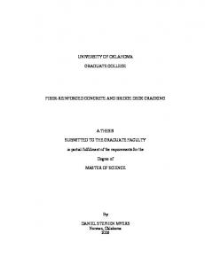
Fig. 1 shows a 2D close-packed particle lattice. Each particle is spaced a distance, s, from its six nearest neighbors.

√3 s 2

y

x

𝑁

𝑖 ∑𝑗=1 𝑭𝒊𝒋 + 𝑭𝒆𝒙𝒕𝒊 = ∆𝑚𝒖̈ 𝒊 ,

𝑁𝑖 ∑𝑗=1 𝑴𝒊𝒋 + 𝑴𝒆𝒙𝒕𝒊 = ∆𝐼𝜽̈𝒊 ,

and

s

(1) (2)

where 𝑭𝒊𝒋 and 𝑴𝒊𝒋 are the force and moment vectors, respectively, exerted by particle j on particle i, 𝑭𝒆𝒙𝒕𝒊 and 𝑴𝒆𝒙𝒕𝒊 are the externally applied force and moment vectors, respectively, applied to the centroid of particle i, and 𝒖̈ 𝒊 and 𝜽̈𝒊 are the linear and angular acceleration vectors, respectively, of the centroid of particle i. 𝑁𝑖 is the number of particles, j, that are within the spherical neighborhood, whose radius is the “material horizon”, 𝛿, of particle i. With a close-packed lattice, and 𝛿 = 1.5𝑠, 𝑁𝑖 is six (or less) for a 2D problem. Of course, one could contemplate MPLM models with larger material horizons, which might be preferable from the point of view of producing isotropic damage behavior with respect to lattice orientation, but the number of neighboring particles, 𝑁𝑖 , and thus the number of force computations would be larger, per particle. Equations 1 and 2 are integrated explicitly in time using the velocity Verlet integration method, with time step, Δ𝑡 = 𝑠/(𝑛 × 𝑐0 ), with s being the particle spacing, 𝑐0 being the speed of sound in the material, and n being π or greater for stability. Because we are interested in modeling cementitious materials, with highly nonlinear material behavior, explicit time integration is the method of choice. The vector functions 𝑭𝒊𝒋 and 𝑴𝒊𝒋 describe the internal forces and moments between neighboring lattice particles, and from these

Figure 1: Two-dimensional hexagonal lattice.

The volume per particle is ∆𝑉 = √3 𝑠 2 𝑡 for a 2 2D hexagonal lattice representing a flat plate of thickness, t. To represent a material with a mass density of ρ, each particle is endowed with a mass of ∆𝑚 = 𝜌∆𝑉. Assuming that each particle is a uniform solid sphere with radius, 𝑠 𝑟 ≈ , its mass moment of inertia, ∆𝐼 , identical 2 about all axes through the particle, is ∆𝐼 = 2 𝑚𝑟 2 . 5 The particle lattice spacing, s, can reasonably be chosen as the material grain characteristic size (such as the maximum aggregate size for concrete). Alternately particle spacing, s, may be chosen based upon the requirement that the number of particles used for a particular problem not exceed the capacity of the computational resource. For a material like concrete, it makes no sense to allow the particle lattice spacing to be less than the aggregate size; the mesoscale of the material sets a lower bound on appropriate lattice particle spacing, s. Indeed, it makes no sense to define geometric features that are smaller than the aggregate size, as even if a structure with such small features could be constructed, these tiny features could hardly be considered as consisting of a spatially homogenous material. Thus, in contrast with 2


spaced at distance s is thought of as a linear elastic Euler-Bernoulli frame element with axial stiffness a=E’A and bending stiffness b=E’I, then to simulate a plane-stress elastic continuum of thickness t and with Young’s modulus E and Poisson’s ratio, ν, the formulas for a and b are given by

functions, the material behavior emerges. For a bond-based micropolar peridynamic model, 𝑭𝒊𝒋 and 𝑴𝒊𝒋 are chosen to be functions of the reference position vectors, 𝒙𝟎𝒊 and 𝒙𝟎𝒋 , and current position vectors, 𝒙𝒕𝒊 and 𝒙𝒕𝒋 , and also as functions of the velocities 𝒗𝒕𝒊 and 𝒗𝒕𝒋 of particles i and j. Note that all of these kinematic vectors include particle positions (and velocities) as well as particle rotations (and angular velocities). The functions 𝑭𝒊𝒋 and 𝑴𝒊𝒋 also depend upon evolving damage parameters, 𝜔𝑖𝑗 , associated with the interaction between particle i and particle j. For a state-based peridynamic model [4], vectors 𝑭𝒊𝒋 and 𝑴𝒊𝒋 may be functions not only of the states of particles i and j, but also of all other particle, k, states and interaction damage states, 𝜔𝑖𝑘 , within the peridynamic horizon of particle i. With today’s high performance parallel computers, a million particles can reasonably be modeled, and for concrete with aggregate 3 size of 2 cm, a volume of (0.02𝑚) �𝑝𝑎𝑟𝑡𝑖𝑐𝑙𝑒 ×

𝑎=

√3(1−𝜈)

𝐸𝑠3 (1−3𝜈)𝑡

and 𝑏 = 12√3(1−𝜈2 ) .

(3)

Similar expressions for 1D, 2D plane strain, and 3D continua are found in [5]. In our computational formulation, elastic interaction deformations (interaction stretches and curvatures) are assumed to be reasonably small, but large translations and rotations are accounted for using a co-rotational stiffness formulation [6; 7]. Thus, patches of particles can detach as rigid bodies and move correctly with large translations and rotations. However, particle collision behavior is not currently incorporated into the model, except between particles that are adjacent in the reference lattice. While the presented linear elasticity model gives the same results as the classical NavierCauchy elasticity model for states of uniform strain far from boundaries, it yields slightly different results than the classical elasticity model in the presence of nonuniform strain fields and near boundaries. This does not make the MPLM model wrong; just slightly different than the Navier-Cauchy continuum model. One could argue that the MPLM elasticity model is more realistic than the classical Navier-Cauchy model for materials like concrete.

1,000,000 𝑝𝑎𝑟𝑡𝑖𝑐𝑙𝑒𝑠 = 8𝑚3

of concrete for at least several fundamental vibration periods can be simulated. Thus, on a parallel computer, it is feasible to simulate large 3D concrete structures using the MPLM – not just small laboratory specimens. In solid models, the forces between particles are assumed to arise due to deviations from a reference state. As long as the deviation of particle positions from their reference locations is not too extreme, the MPLM is suitable. Taking the terminology “cohesive crack model” to its logical conclusion, the MPLM could perhaps be termed a “cohesive particle” model. 3

𝐸𝑠𝑡

3.2 MPLM damage model With reference to Fig. 2, the micropolar axial stretch of interaction ij,

MPLM MODEL FOR CONCRETE

A MPLM constitutive model for concrete is proposed in this section. Others are certainly possible. We start with the linear elastic regime.

𝜖𝑎 ≡

𝑑𝑡 −𝑑 𝑑

,

(4)

where 𝑑𝑡 is the current length and d is the reference length, is defined in a manner similar to axial strain. Similarly, the maximum micropolar

3.1 MPLM linear elasticity If the interaction between two particles 3


curvatures about the local z-, y- and x-axes, respectively, of interaction i j are: 2

3

𝑗

� �2𝜃𝑧𝑖 + 𝜃𝑧 −

𝑗

�𝑑𝑦 − 𝑑𝑦𝑖 �� , �, 𝜓𝑧 ≡ 𝑚𝑎𝑥 � 2 3 𝑗 𝑗 � �2𝜃𝑧 + 𝜃𝑧𝑖 − �𝑑𝑦𝑖 − 𝑑𝑦 �� 𝑑

𝑑

2

𝑑

𝑑

𝑗

� �2𝜃𝑦𝑖 + 𝜃𝑦 −

3

𝑗

�𝑑𝑧 − 𝑑𝑧𝑖 �� , �, and 𝜓𝑦 ≡ 𝑚𝑎𝑥 � 2 3 𝑗 𝑗 � �2𝜃𝑦 + 𝜃𝑦𝑖 − �𝑑𝑧𝑖 − 𝑑𝑧 �� 𝑑

𝑑

𝜓𝑥 ≡ �

𝑗

𝜃𝑥 −𝜃𝑥𝑖 𝑑

�

𝑑

parameter for interaction ij in the immediately preceding time step. The damage function Ω𝑡 �𝜖𝑚𝑝+ � is defined in Fig. 3(a), and it has been chosen in such a way that the cohesive tensile softening behavior is modeled approximately correctly.

(5)

(6)

𝑑

.

(7)

We propose measures of micropolar tensile and compressive interaction deformation as 𝜖𝑚𝑝+ ≡ 𝜖𝑎 + 𝛽𝑑�𝜓𝑥 2 + 𝜓𝑦 2 + 𝜓𝑧 2

and

𝜖𝑚𝑝− ≡ 𝜖𝑎 − 𝛽𝑑�𝜓𝑥 2 + 𝜓𝑦 2 + 𝜓𝑧 2 ,

(8) Figure 3: (a) Damage, 𝜔𝑡 , versus the micropolar strain measure, 𝜖𝑚𝑝+ . (b) Damage, 𝜔𝑐 , versus the micropolar

(9)

strain measure, 𝜖𝑚𝑝− . (𝜔𝑡 and 𝜔𝑐 never decrease with time.)

where β is a dimensionless parameter.

For the evolution of compression damage, 𝜔𝑐 : for 𝜖𝑚𝑝− ≤ 𝛼𝑐 𝜖𝑐 , 𝜔𝑐 = 1 for 𝛼𝑐 𝜖𝑐 ≤ 𝜖𝑚𝑝− ≤ 𝜖𝑐 ,

𝜔𝑐 = max�Ω𝑐 �𝜖𝑚𝑝− �, 𝜔𝑐𝑝𝑟𝑒𝑣 �

Figure 2: Displacement and force components, in local coordinates, acting between particles i and j, separated by reference distance, d.

for 𝜖𝑐 ≤ 𝜖𝑚𝑝− ,

for tension damage:

for 𝜖𝑡 ≤ 𝜖𝑚𝑝+ ≤ 𝛼𝑡 𝜖𝑡 ,

𝜔𝑡 = 𝑚𝑎𝑥�0, 𝜔𝑡𝑝𝑟𝑒𝑣 �

𝜔𝑡 = 𝑚𝑎𝑥�Ω𝑡 �𝜖𝑚𝑝+ �, 𝜔𝑡𝑝𝑟𝑒𝑣 �

for 𝛼𝑡 𝜖𝑡 ≤ 𝜖𝑚𝑝+ ,

𝜔𝑡 = 1 ,

and

(14)

𝜔𝑐 = max�0, 𝜔𝑐𝑝𝑟𝑒𝑣 �,

(15)

where 𝜔𝑐𝑝𝑟𝑒𝑣 is the value of the compressive damage parameter for interaction ij in the immediately preceding time step. Function Ω𝑐 �𝜖𝑚𝑝− � is defined in Fig. 3(b). The damage parameter, ω, is computed as the maximum of 𝜔𝑡 and 𝜔𝑐 . If 𝜖𝑎 ≥ 0, then

The tensile damage parameter, 𝜔𝑡 , is defined in terms of these deformation measures, with reference to Fig. 3, as:

for 0 ≤ 𝜖𝑚𝑝+ ≤ 𝜖𝑡 ,

(13)

(10)

{f}=(1- ω)[K]{d}

,

(16)

{f}=(1- ω )[K*]{d} ,

(17)

and if 𝜖𝑎 ≤ 0, then

and (11) (12)

where {f} is the force vector acting between

where 𝜔𝑡𝑝𝑟𝑒𝑣 is the value of the tensile damage 4


𝑗

compressive axial force (𝑓𝑥𝑖 = −𝑓𝑥 ). For equilibrium with the shear force, the moments

particles i and j, [K] is the elastic stiffness matrix defined using Eq. 3, and {d} is the vector of particle deformations, associated with interaction ij. Because there are many interactions per particle, this form allows damage to be anisotropic. With the stiffness matrix, [K*], the axial components of force are the same as that computed by [K], but the shears and moments are reduced by the damage parameter (1-ω). Thus, compression failure is indirectly precipitated by loss of moment and shear capacity (and subsequent instability due to nonlinear geometric effects), but not by loss of axial stiffness. In this implementation, damage can be either tensile or compressive, but not both. The constitutive model presented has eight parameters: peridynamic lattice spacing parameter s, micro-elastic stiffness parameters a and b, and the parameters governing tensile and compressive damage evolution: 𝜖𝑡 , 𝛼𝑡 , 𝜖𝑐 , 𝛼𝑐 , and 𝛽 . The lattice spacing parameter, s, is chosen to be as small as the available computational capacity allows, but no less than the largest material grain size. The parameter 𝜖𝑡 is calibrated to reproduce the tensile strength, 𝑓𝑡 , of the concrete: 𝜖𝑡 ≈ 𝑓𝐸𝑡. The parameter, 𝛽 ≈ 0.1, is chosen to replicate the ratio of uniaxial compressive load to uniaxial tensile load, usually around ten, as is observed empirically for normal-strength concrete. The parameter 𝑠𝑐 ≈ 0.001 is chosen to replicate the strain at which uniaxial compressive failure commences, and 𝛼𝑐 𝑠𝑐 ≈ 0.003 is chosen to represent the ultimate compressive strain. The parameter 𝛼𝑡 is chosen to replicate the tensile fracture energy, 𝐺𝐹 , of the material, as described in [1].

𝑗

are computed as 𝑚𝑧𝑖 = 𝑚𝑧 =

3.4 MPLM damping model

𝑑𝑓𝑖𝑦 2

.

Damage events can release sudden bursts of acoustic energy. If no material damping is included in the model, this acoustic energy can cause spurious vibration and consequent damage. Thus we incorporate an axial peridynamic damping model. When computing the force in interaction ij, the relative axial velocity, 𝑣𝑖𝑗 , between particles i and j is computed. Then the axial damping force, 𝑓𝑑𝑎𝑚𝑝𝑖𝑗 , between the two particles is given by 𝑓𝑑𝑎𝑚𝑝𝑖𝑗 = 2𝜁𝑚𝜔𝑛 𝑣𝑖𝑗 , and 𝐹𝑖𝑗 = 𝑓𝑒𝑙𝑎𝑠𝑡𝑖𝑗 + 𝑓𝑑𝑎𝑚𝑝𝑖𝑗 ,

(18) (19)

where 𝜁 is the ratio of critical damping, with value set between 0 and 1, 𝑚 is the particle mass, 𝜔𝑛 is the highest natural frequency of vibration, 𝑣𝑖𝑗 is the relative axial velocity between particles i and j, 𝑓𝑒𝑙𝑎𝑠𝑡𝑖𝑗 is the elastic inter-particle axial force calculated in the previous section, including the effect of damage, and 𝐹𝑖𝑗 is the internal axial force used in Eq. 1. The damping force, always opposing the direction of motion, removes energy from the system. We find that choosing 𝜁 ≈ 0.05 produces reasonable damping behavior. A similar strategy, not yet implemented and apparently not necessary, may be used to damp shear and rotational degrees of freedom. 4 MODELING OF REINFORCING BARS AND BOND A reinforcing bar is represented as a 1D lattice of MPLM particles representing a bar with cross-sectional area As and crosssectional moment of inertia Is. The material parameters are Young’s modulus Es and yield stress Fy. Steel particles interact if they spaced less than s from each other. Steel particles from separate reinforcing bars do not interact. As shown in Fig. 4, only every other steel

3.3 MPLM frictional model The frictional model requires that when the link is in axial compression (𝜖𝑎 ≤ 0), and when 𝜔=1 the magnitude of the shear force 𝑗 𝑖 (𝑓𝑦 = −𝑓𝑦 ) must never exceed the internal coefficient of friction, µ, times the 5


The steel-concrete MPLM interactions are identical to concrete-concrete interactions, except that they are assumed to be linear elastic, with no damage. The steel is modeled as elastic-perfectly plastic.

particle of a given rebar is connected to concrete particles within a horizon s using the same elastic interaction model as for concreteconcrete particles (such interactions assume no damage). The reason that only every other steel particle is connected to concrete is to allow cracks in concrete to develop unhindered by the non-damaged steel-concrete interactions. If the distance between a steel particle and a concrete particle is zero, the interaction between these two particles is ignored.

Table 1: Classical material parameters

Figure 4: Bond of reinforcement (red) to concrete (black) using peridynamic interactions (tan).

Value

Units

Conc. Young’s modulus, Ec

24.86

GPa

Conc. Poisson’s ratio, µc Conc. comp. strength, f’c

0.20

-

27.58

MPa

Conc. tens. strength, ft

2.758

MPa

Conc. Density, ρc

2323.0

kg/m3

Conc. fracture toughness, GF

175.0

N/m

Steel Young’s modulus, Es

200.0

GPa

Steel yield strength, Fy

414.0

MPa

Steel Poisson’s ratio, µs

0.3

MPa

Steel Density, ρs

7850.0

kg/m3

Table 2: MPLM parameters for concrete

Parameter Lattice Spacing, s Microelastic parameter, a Microelastic parameter, b Tensile stretch limit St Tensile stretch ratio αt Sc αc β Damping ratio, c

Bond-slip is indirectly modeled and emerges from the elasticity and damage of the interactions between surrounding the concrete particles. 5

Parameter

EXAMPLES

In all of the following examples, the target classical materials parameters are shown in Table 1, and the corresponding selected MPLM parameters for concrete and steel are shown in Tables 2 and 3. The time step is 𝑠 = 1.808 × 10−7 𝑠. chosen as ∆𝑡 = 24𝑐

Value 0.020 4.557x107 506.3 0.000126 10 -0.001 5.728 0.10 0.05

Units m N N-m2 -

Table 3: MPLM parameters for steel

Parameter Lattice Spacing, s Microelastic parameter, a Microelastic parameter, b Yield limit, St Damping ratio, c

0(𝑠𝑡𝑒𝑒𝑙)

In each example, the load is linearly ramped from zero to the peak load for duration of at least four fundamental periods of the structure, and is thus essentially quasistatic. The load is ramped from time zero up to 75% of the total simulation time and then held constant. “Strength” is defined as the peak load at which static equilibrium can still be achieved. In all of the following examples, the particles in the deformed configuration are shown and the damaged interactions are colorcoded as shown in Fig. 5. Undamaged interactions are not shown in the figures.

Value 0.020 EsAs EsIs 0.00207 0.05

Units m N N-m2 -

Concrete particles Steel particles Tensile damage (0