Sep 11, 2012 - 2-star statistics and triad closure using triangle counts as suggested in Frank ..... tions With Network Structure,â Scandinavian Journal of Statistics, 29, 375â390. ... Fellows, I., and Handcock, M. S. (2012), âExponential-family ...
Computational Statistical Methods for Social Network Models David R. Hunter, Pavel N. Krivitsky, and Michael Schweinberger∗ September 11, 2012
Abstract This article reviews the broad range of recent statistical work in social network models, with particular emphasis on computational aspects of these methods.
Keywords: degeneracy, ERGM, latent variables, MCMC MLE, variational methods
1
Introduction
A typical statistical data frame includes sampling units, which may be considered individuals, and analysis often focuses on some property of these units. Loosely speaking, social networks arise whenever the “property” of interest involves interactions between multiple sampling units, rather than the units themselves. We do not limit ourselves to the case in which the sampling units are actually human beings, though this is by far the most common application that has appeared in the literature on social network models. There is a long history of work that may be characterized as related to social networks—as Carrington and Scott (2011) point out, it is difficult to pinpoint the genesis of this field but its roots may be traced at least as far back as the 1930s—though we do not focus on this development here, both because there already exist numerous treatises on networks in general and social networks in particular, and because for the audience of JCGS, we wish to focus on computational questions. However, we can at least give a partial list of survey-type references for readers interested in delving into the subject of social networks more deeply: Though almost two decades old, the ∗
All three authors contributed equally to this article.
1
classic book by Wasserman and Faust (1994) is still considered a comprehensive introduction to the important quantitative concepts of social network analysis. As to statistical analysis for social networks, more recent works include the survey article by Goldenberg et al. (2009) and the booklength treatment of various network-related statistical topics by Kolaczyk (2009), both of which give numerous references. Finally, we recommend the other network-related articles in this issue. The current article highlights some current topics in social network modeling, with special emphasis on computational aspects. In Section 2, we introduce a classic dataset, which, though extremely small especially by modern standards, serves to illustrate some of these computational techniques even if it does not demonstrate the state-of-the-art in computational techniques designed for massive social networks. To keep the article to a manageable length, in Section 3 we merely highlight many important topics illustrating the range of statistical work on social network applications, citing recent references to enable interested readers to learn more. The topics that we describe in more detail in Sections 4 and 5 share a common feature: they focus on complete networks that are cross-sectional, which means that they observed at only one point in time. The distinction between the techniques in Section 4 and those in Section 5 is that the former covers network models whose dependence structure does not have a clear hierarchy, typically expressed as a joint distribution of edge variables, and often focused on modeling global network features and social forces; whereas the latter covers network models that are hierarchical in nature, where the edge variable distributions are parameterized in terms of latent variables, and are focused on identifying individual nodes’ roles and positions. We conclude in Section 6 with a discussion of some future challenges. Our hope throughout is to stimulate interest among the readership of JCGS to delve into the rapidly expanding field of statistical modeling of social networks.
2
Data and notation
We introduce some notation used throughout the article and then discuss a classic social network data set, which we use as an illustrative example throughout the paper.
2
2.1
Notation
Let N be the set of nodes in the network of interest, indexed {1, . . . , n}. The relationships in the network may be directed (e.g., friendship nominations, messages) or undirected (e.g., sexual partnerships, conversations). In the former case, we define the set of dyads (here used to refer to potential relationships) Y to be a subset of N × N , the set of ordered pairs of nodes; in the latter case, it is a subset of {{i, j} : (i, j) ∈ N × N }, the unordered pairs of nodes. (We will also use u(Y) to refer to an “unordered” version of Y, i.e., u(Y) ≡ {{i, j} : (i, j) ∈ Y}.) Usually, Y is further constrained in that in most social networks studied, a node cannot have a relationship of interest with itself, excluding pairs of the form (i, i). For binary networks, in which the relationship of interest must be either present or absent, we use Y ⊆ 2Y , the set of subsets of Y, to refer to the set of possible networks of interest, which may be further constrained (that is, Y may be a proper subset of 2Y ). We will use Y to refer to network random variables and y ∈ Y to refer to their realizations, and yi,j be an 0–1 indicator of whether a relationship of interest is present between i and j in a binary network context.
2.2
Data
The data set collected by Sampson (1968) and described by Batagelj and Mrvar (2003) is a classic data set in social network analysis. The data set summarizes relationships, observed at three distinct time points, among 18 monks who were about to enter a monastery when a conflict erupted. We use here the directed network where yi,j = 1 denotes that monk i liked monk j at any of the three time points and yi,j = 0 otherwise. The directed network is shown in Figure 1, where circles represent monks and directed edges are oriented from i to j whenever yi,j = 1. The monks are divided by Sampson into three groups: Loyal Opposition, Turks, and Outcasts.
3
Range of social network models
The range of statistical modeling techniques for social networks is too broad to address adequately in a single article. We have chosen to focus in some depth in Sections 4 and 5 on cross-sectional
3
Loyal
Turks
Outcasts
Figure 1: Monk social network dataset of Sampson (1968), where circles represent monks and directed edges represent liking relationships. (i.e., observed once only), completely observed networks. The current section, by contrast, seeks to illuminate the myriad other applications by describing several additional important recent trends in social network modeling for which we do not have space for a lengthier exposition.
3.1
Dynamic Markovian models of networks
The modeling of social network dynamics—i.e., changes over time—has attracted much attention, starting with the groundbreaking work of Holland and Leinhardt (1977a,b) and Wasserman (1977, 1979, 1980). Holland and Leinhardt argued that continuous-time Markov processes with state space Y are natural models of social network dynamics. Wasserman’s work, later sharpened by Leenders (1995), studied maximum likelihood estimation for continuous-time Markov process models based on the assumptions that dyad processes are independent and stationary. This early work was expanded by Snijders (2001), who introduced parameterizations of continuoustime Markov processes that allow dyad processes to be dependent and relaxed the restrictive stationarity assumption provided two or more discrete-time observations of the process are available. Motivated by the work of McFadden (1974) on random utility models, Snijders’ parameterizations have the advantage that the Markov process can be interpreted as “actor-driven”, i.e., driven
4
by nodes who maximize random utility functions of the network. More importantly from the standpoint of statistical computing, Snijders (2001) also adapted the method of simulated moments (McFadden, 1989) to method of moments estimation of continuous-time Markov models, implemented by stochastic approximation (Robbins and Monro, 1951; Pflug, 1996). Some computational improvements were discussed by Schweinberger and Snijders (2007), and maximum likelihood and Bayesian estimation were proposed by Snijders et al. (2010) and Koskinen and Snijders (2007), respectively. These computational methods are based on non-standard (Markov chain) Monte Carlo data-augmentation methods and are implemented in the Windows-based program Siena (Snijders et al., 2010a) and the platform-independent R package RSiena (Ripley and Snijders, 2011). More recently, discrete-time Markov models have been explored as alternatives to continuoustime Markov models. Hanneke et al. (2010) explored discrete-time Markov models in which the transition probabilities are expressed by ERGMs. Krivitsky and Handcock (2012a) proposed separable parameterizations of discrete-time Markov models, where one process governs the addition of edges and the other process governs the deletion of edges at each time step; their estimation methods, which extend the (Markov chain) Monte Carlo maximum likelihood methods of Geyer and Thompson (1992), are implemented in the R package ergm package (Handcock et al., 2012).
3.2
Dynamic non-Markovian models of networks
Several non-Markovian models for changing networks, including loglinear models and models in which changes are selected uniformly conditional on the degree structure of the network, are discussed briefly by Frank (1991), who cites multiple references. A more recent method is the random-effects model suggested by Westveld and Hoff (2011), which may be adapted to network data that are either binary or in which edges between nodes have normally distributed weights. One recent trend in the non-Markovian vein in which computation plays an increasingly important role is the application of survival analysis to continuously collected network data (Butts, 2008; Brandes et al., 2009), an increasingly common paradigm with internet-based and other computer-generated network datasets. If an “event” is the formation of a new edge, then we
5
attach a counting process either to every node or to every pair of nodes. Vu et al. (2011) refer to these as the “egocentric” and “relational” models, respectively. The analysis of large datasets (with thousands of nodes and tens of thousands of edges) based on these counting processes is demonstrated in the egocentric case by Vu et al. (2011) and in the relational case by Vu et al. (2011) and Perry and Wolfe (2011).
3.3
Joint models of networks and other outcome variables
There is a growing literature in which statistical models for the edges in a network are only one part of a larger joint model. Computing plays a huge role in this area, as simulations of these joint models are vital; yet statistical inference is a relatively recent addition to the computational mix. Snijders et al. (2007), for instance, model jointly a dynamically evolving network along with behavior measured on the nodes in that network; parameter estimation for such models given longitudinally observed data is implemented in SIENA (Snijders et al., 2010a; Ripley and Snijders, 2011). Fellows and Handcock (2012) demonstrate the computational viability of models in which covariates on the nodes in a network are considered random variables. An important subclass of these joint models are models in which a social network is modeled together with some other process of interest that takes place among the nodes in the network, as in the study of infectious diseases. For instance, Britton and O’Neill (2002), whose models were later extended and applied by Groendyke et al. (2011, 2012), use an MCMC-based Bayesian approach to infer model parameters for a contact network underlying an outbreak of an infectious disease when certain information is available about the outbreak, even in cases where none of the contact network edges is actually observed.
3.4
Measurement error models and partially sampled networks
Accuracy of network data may be suspect for a number of reasons. A vast sociological literature on the question of how reliable respondents’ reports might be has failed to resolve the question; yet even if it is not quite true that “[self-report] data about communication cannot be used as a proxy for behavioral data” (Bernard et al., 1979), the statistical community will certainly not
6
be surprised to learn that noise in data collection, along with missing data, can pose significant problems in data analysis. Butts (2003) explores this theme from a statistical point of view, advancing a hierarchical Bayesian framework for simultaneously analyzing network structure along with respondent accuracy. Wyatt et al. (2008) report promising results inferring parameters for a network model from noisy data using a stochastic gradient ascent algorithm to optimize the computationally intractable likelihood function. An important subcategory of models for which data are imperfectly observed are those in which some (known) portion of the network observations is missing. Both maximum likelihood (Gile and Handcock, 2010) and Bayesian (Koskinen et al., 2010) approaches to this missing-data problem have been proposed and demonstrated to be viable, though each relies heavily on computational techniques: Both use MCMC to help approximate an intractable likelihood, while the latter also uses Bayesian data augmentation.
4
Exponential-family random graph models: global network characteristics
In this section, we discuss models represented in terms of the joint distribution of all edges, as opposed to a series of conditional distributions of a hierarchical model as described in Section 5. The most popular framework for these joint models is the class of exponential-family random graph models (ERGMs). Originally proposed by Holland and Leinhardt (1981) to model individual heterogeneity of nodes and reciprocity of their edges (called the p1 model), the framework was generalized by Frank and Strauss (1986), Wasserman and Pattison (1996) (who called it the p∗ model), and Snijders et al. (2006). It takes the form of a (curved) exponential family on the sample space Y: Pθ (Y = y) =
exp{η(θ)> g(y)} , y ∈ Y, κ(θ)
(1)
where θ is a q-vector of model parameters, which are mapped to a p-vector of natural parameters by η(·); and g(·) is a p-vector of sufficient statistics, which capture network features of interest, its postulated dependence structure, or both. We present some examples of ERGM statistics in
7
Edges
t
g(y)
-t
X (i,j)∈Y
∆i,j g(y)
Mutual dyads
yi,j
t�
-t
X
yi,j yj,i
Transitive triads t �� A � � t�
X
(i,j)∈u(Y)
1
(i,j)∈Y
X
yj,i
yi,j
A A -AU t
X
yi,k yk,j
k∈N \{i,j}
(yi,k yk,j + yi,k yj,k + yk,i yk,j )
k∈N \{i,j}
Table 1: Well-known network statistics, where circles represent nodes and directed lines represent directed edges between nodes. The first two of these statistics are used in the model of Section 4.4, whereas the last is replaced in the models by a statistic that is less prone to the degeneracy problem discussed in Section 4.3.
Table 1. Lastly, to make all probabilities sum to one, κ(θ) =
X
� exp η(θ)> g(y 0 ) .
y 0 ∈Y
Notably, this differs from the “textbook” exponential family formula, in that it omits an “h(y)” factor, which, together with Y, controls the “reference measure” for the model, the distribution of networks when η(θ) = 0. While usually omitted in binary ERGMs, it gains a great deal of importance when using exponential families to model valued networks ties (Krivitsky, 2012). Exponential families for networks can be derived by postulating a substantively relevant conditional dependence structure, and, based on this structure, approaches like the Hammersley-Clifford Theorem (Besag, 1974) can be used to derive sufficient statistics associated with the model. Frank and Strauss (1986) derive a set of statistics under the “Markovian” assumption that the states of two relationships are, conditional on the rest of the network, stochastically dependent only if they have at least one node in common. Other examples of this approach include the work of Pattison and Wasserman (1999) on multivariate relations, Robins et al. (1999) on polytomous relations, and the realization-dependent conditional independence of Snijders et al. (2006). At the same 8
time, choice of statistics can be driven by beliefs about the factors that influence the underlying social process, without regard for dependence structure (Morris et al., 2008; Krivitsky, 2012). For each dyad, one can derive its conditional distribution given the rest of the network, i.e., �� � exp{η(θ)> g(y + (i, j))}/� κ(θ) > = exp η(θ) ∆ g(y) , Oddsθ (Y i,j = 1 | Y −(i, j) = y −(i, j)) = i,j �� exp{η(θ)> g(y − (i, j))}/� κ(θ) with ∆i,j g(y) ≡ g(y ∪ {(i, j)}) − g(y\{(i, j)}), the change in the sufficient statistic vector associated with adding an edge at (i, j). These “change statistics” (Hunter and Handcock, 2006) or “change scores” (Snijders et al., 2006) facilitate “local” interpretation of ERGMs. For example, consider the mutual dyads statistic in Table 1: θ↔ associated with this statistic can be said to increase the conditional odds of an edge (i, j) by exp{θ↔ } if there is already a tie from j to i. When ∆i,j g(y) does not depend on y, the model is dyad-independent, and can be decomposed into logistic regression for each edge.
4.1
Simulation methods
Many applications of these models, including all of the Monte Carlo-based methods for finding a maximum likelihood estimator (MLE) as well as Bayesian methods, require making draws from the ERGM. Because evaluating the conditional probability of an edge given the rest of the network is often relatively inexpensive, it is straightforward to simulate network realizations even from intractable ERGMs using a Metropolis-Hastings sampling procedure: given a proposal y´ from density q(y´ | y), accept with probability �� � ´ exp{η(θ)> g(y)}/ ´ � ´ q(y | y) κ(θ) q(y | y) ´ − g(y)) = exp η(θ)> (g(y) � > � q(y´ | y) exp{η(θ) g(y)}/� κ(θ) q(y´ | y) P or 1, whichever is smaller. Supposing that q(y´ | y) > 0 only if (i,j)∈Y I (y´i,j 6= yi,j ) equals one—
´ − g(y) i.e., the proposed network is constructed by toggling a single edge, say (i, j)—then g(y) reduces to ±∆i,j g(y), with the sign depending on the direction of the toggle, facilitating a fast Gibbs sampling algorithm. Morris et al. (2008) further optimize it for large, sparse networks by implementing an asymmetric proposal. The rate of convergence for this Gibbs procedure was studied by Bhamidi et al. (2008). There is also some work in progress on exact sampling (Butts, 2012). 9
4.2
Inference methods
The major challenge associated with applying these models is the intractability of the normalizing constant κ(θ) in the likelihood. Here, we describe the methods used to address this challenge. 4.2.1
Pseudo-likelihood estimation
An approximate approach to maximum likelihood estimation is based on the so-called pseudolikelihood function (Strauss and Ikeda, 1990), defined as Y
Y � Pθ Y i,j = yi,j | Y \{(i, j)} = y\{(i, j)} =
(i,j)∈Y
(i,j)∈Y
1 ≈ Pθ (Y = y). 1 + exp{−θ > ∆i,j g(y)}
In other words, for each potential edge in the network, its conditional probability given the state of the rest of the network is evaluated, and the product of those probabilities is used to approximate the likelihood. Maximizing the pseudo-likelihood results in a maximum pseudo-likelihood estimator (MPLE), which, computationally, reduces to logistic regression (Strauss and Ikeda, 1990). van Duijn et al. (2009) and others show that the MPLE is often biased and far less efficient than the MLE, particularly when the social process modeled has strong dyadic dependence, and is particularly vulnerable to the “degeneracy” issues discussed below. van Duijn et al. (2009) also propose a maximum bias-corrected pseudolikelihood estimator (MBLE). 4.2.2
Maximum likelihood estimation: stochastic approximation
In the case of linear ERGMs, the maximum likelihood estimator of θ solves ∇θ log Pθ (Y = y) = g(y) − Eθ (g(Y )) = 0,
(2)
where ∇θ log Pθ (Y = y) denotes the gradient of the log likelihood function log Pθ (Y = y) with respect to θ. Snijders (2002) proposes solving equation (2) using stochastic approximation (Robbins and Monro, 1951; Pflug, 1996). Starting with an initial guess, the stochastic approximation method updates θ t to θ t+1 at iteration t + 1 as follows: ˆ t−1 (g(Yθt ) − g(y)), θ t+1 = θ t − at D
10
where Dt−1 is an approximation of the gradient ∇θ Eθ (g(Y )) in the neighborhood of θ t , at is a sequence of numbers which tends sufficiently slowly to 0 as t increases, and Yθt is a network sample from the ERGM with parameter θ t by Markov chain Monte Carlo (MCMC) methods. Okabayashi and Geyer (2012) propose a linear search algorithm along similar lines, while Jin and Liang (2012) develop yet another stochastic approximation algorithm. 4.2.3
Maximum likelihood estimation: Monte Carlo maximization
An alternative approach to maximum likelihood estimation is based on Monte Carlo approximations of the likelihood function (1). The MCMC MLE approach of Geyer and Thompson (1992) was first adapted by Handcock (2003) to ERGMs and extended by Hunter and Handcock (2006). Both the stochastic approximation algorithm of Snijders (2002) described in Section 4.2.2 and the MCMC MLE approach of Hunter and Handcock (2006) rely on MCMC simulations of networks, but the MCMC MLE approach has the advantage that it makes more efficient use of MCMC samples, as pointed out by Geyer and Thompson (1992, Section 1.3). Starting with an initial guess θ, which is often taken to be the easy-to-calculate MPLE, the ratio of intractable normalizing constants is approximated as n o exp{η(θ)> g(y)} κ(θ 0 ) X > = exp (η(θ 0 ) − η(θ)) g(y) κ(θ) κ(θ) y∈Y � n o� > = Eθ exp (η(θ 0 ) − η(θ)) g(Y ) , with the last expectation approximated by a sample of sufficient statistics under θ, allowing the likelihood to be maximized as a function of θ 0 . In practice, the accuracy of the estimate decreases as θ 0 moves farther from θ; in particular, if a guess θ is so far from the MLE that the interior of the convex hull of a sample under θ does not contain the observed sufficient statistic, the maximized θ 0 does not exist (Hummel et al., 2012). Thus, practical implementation such as that of Handcock et al. (2012) involves several iterations of refining the guess and sampling from it. The MPLE is often used for the purpose, and Okabayashi and Geyer (2012) suggest using their linear search algorithm for the purpose, while Hummel et al. (2012) propose an adaptive method to attenuate the change in θ 0 . 11
Publicly available implementations of ERGM MLE and MPLE include the ergm package (Hunter et al., 2008; Handcock et al., 2012) from the Statnet suite of R packages and PNet (Wang et al., 2009). 4.2.4
Bayesian methods
Bayesian inference is based on the posterior distribution of θ given y: p(θ | y) = where p(y) =
R
p(y | θ) p(θ) p(θ, y) = ∝ p(y | θ) p(θ), p(y) p(y)
p(y | θ) p(θ) d θ is the marginal probability of y, p(y | θ) = Pθ (Y = y) is the
conditional probability of y given θ, p(θ) is the prior probability density of θ, and p(θ | y) is the posterior density of θ given y. The posterior density p(θ | y) is typically intractable, because its normalizing constant p(y) is intractable. Standard MCMC methods, e.g., the Metropolis-Hastings algorithm, can deal with intractable normalizing constants of a posterior density as long as the posterior density in question is known up to a constant. The problem is that the posterior density is not known up to a constant, because the normalizing constant κ(θ) of the likelihood function p(y | θ) is intractable. Since the posterior density p(θ | y) of complex ERGMs includes two intractable normalizing constants, p(y) on the one hand and κ(θ) on the other hand, the posterior density is doubly intractable (Murray et al., 2006). To demonstrate that standard MCMC methods cannot sample from doubly intractable posterior densities, suppose that we want to construct a Markov chain with stationary distribution p(θ | y) by a Metropolis-Hastings algorithm. If θ denotes the current value of the parameter and θ´ denotes a proposal of the parameter generated from a proposal density q(. | θ), then θ´ is accepted with probability min(1, a), where a=
´ p(θ) ´ p(y | θ) . p(y | θ) p(θ)
(3)
´ involve The problem is that acceptance probability (3) is intractable, because p(y | θ) and p(y | θ) ´ respectively. the normalizing constants κ(θ) and κ(θ),
12
A naive approach would be to replace the intractable likelihood ratio by an approximation, either deterministic or stochastic. A deterministic approximation could be based on variational approximations of the log-normalizing constants, while stochastic approximations could be based on MCMC estimators of the ratio of normalizing constants such as the importance sampling estimator used in maximum likelihood estimation (e.g., Murray, 2007). However, the stationary distribution of the resulting Markov chains may not be the desired target distribution, i.e., the posterior density of interest (Murray, 2007). The problematic nature of the naive approach has led to the development of a body of MCMC methods that by design generate samples from doubly intractable posterior density’s. Most of them are based on augmenting the posterior density so that the augmented posterior probability distribution is easy to sample from. We discuss here one of the simplest and most appealing auxiliary-variable MCMC methods, following Murray et al. (2006) and Caimo and Friel (2011). Other auxiliary-variable approaches are discussed by Møller et al. (2006) and Koskinen et al. (2010); an alternative approach, inspired by the Monte Carlo maximum likelihood algorithm of Geyer and Thompson (1992), was proposed by Atchad´e et al. (2012). The basic idea can be described as follows. The data y are augmented by an auxiliary random ´ Suppose the joint density of θ, Y, θ, ´ Y´ is of the graph Y´ and an auxiliary parameter vector θ. form ´ y) ´ ´ = p(θ) p(y | θ) q(θ´ | θ, y) p(y´ | θ), p(θ, y, θ,
(4)
´ is the conditional probability of y´ given θ, ´ where q(θ´ | θ, y) is an auxiliary density and p(y´ | θ) which is of the same exponential-family form as Y , implying the same reference measure and the same sufficient statistics. The augmented posterior density is of the form ´ y´ | y) ∝ p(θ, y, θ, ´ y) ´ ´ ∝ p(θ) p(y | θ) q(θ´ | θ, y) p(y´ | θ). p(θ, θ,
(5)
The posterior density of interest, p(θ | y), is the marginal distribution of the augmented ´ y´ | y). A simple Metropolis-Hastings algorithm to sample from the posterior density, p(θ, θ, augmented posterior density, which has been called the exchange algorithm (Murray et al., 2006; Caimo and Friel, 2011), operates as follows: ´ (1) Sample θ´ | θ, y ∼ q(. | θ, y) and then sample Y´ | θ´ ∼ p(. | θ). 13
(2) Propose to swap the values of θ and θ´ and accept the proposal with probability min(1, a), where a=
´ p(y | θ) ´ q(θ | θ, ´ y) p(y´ | θ) p(θ) . ´ p(θ) p(y | θ) q(θ´ | θ, y) p(y´ | θ)
(6)
´ cancel from Simple calculation shows that the intractable normalizing constants κ(θ) and κ(θ) the acceptance probability (6), so the Metropolis-Hastings algorithm operating on the augmented state space is tractable. Sampling Y´ requires exact sampling, which is typically infeasible. Caimo and Friel (2011) proposed to sample Y´ instead by MCMC methods, as described in Section 4.1. The work of Liang (2010) on double Metropolis-Hastings algorithms provides some justification for doing so. Last, to reduce model degeneracy of conventional ERGMs, Schweinberger and Handcock (2011) proposed hierarchical ERGMs with local dependence and extended the exchange algorithm to hierarchical ERGMs.
4.3
ERGM degeneracy
In addition to the intractable normalizing constant, a major difficulty in modeling complex social processes using ERGMs is a phenomenon referred to as “degeneracy,” which arises for example when attempting to model processes exhibiting individual heterogeneity in activity level using 2-star statistics and triad closure using triangle counts as suggested in Frank and Strauss (1986). In a contemporaneous publication, Strauss (1986) noted that the Markov graph models Frank and Strauss (1986) had proposed tend to, as the network size increases, concentrate an increasingly large probability mass on an increasingly small fraction of possible networks. Jonasson (1999) and H¨aggstr¨om and Jonasson (1999) studied the asymptotics of the so-called triangle model, corresponding to the ERGM with the number of edges and triangles as sufficient statistics, and showed that as the network size increases, the parameter space tends to be divided between configurations that exhibit little triadic closure—typically less than observed—and configurations that are degenerate, in that almost all of the probability mass is concentrated on a single (complete) network. Handcock (2003) and Rinaldo et al. (2009), among others, mapped the shape of the region of the parameter space in which this degeneracy occurred, and Schweinberger (2011) showed that some statistics, including triangle and k-star counts, induce this behavior asymptotically. 14
It can be argued that this degeneracy is merely a symptom of a broader problem of model misspecification. In their development of curved ERGMs, Snijders et al. (2006) used change statistics to show that models with positive coefficients on triangles and/or k-stars induced strong positive dependence among dyad values: edges beget more edges, leading to what the authors called an “avalanche” toward a complete graph. In another realization, the avalanche might not take place, leading to a sparse network. Thus, the model with such positive dependence can induce a bimodal distribution of networks, and, at the MLE, however it is found, the observed network would be between the modes. A bimodal distribution, with little mass between the modes, is difficult for MCMC sampling to explore, which can cause any simulation-based method to fail, whether maximum likelihood or Bayesian. Indeed, Krivitsky (2012), in developing ERGM statistics for networks with weighted edges that are unbounded counts, reports that a statistic analogous to the count of 2-stars induced a bimodal distribution of networks, with neither mode being degenerate (i.e., concentrated) itself. Thus, a fruitful approach to degeneracy may be to model network phenomena using statistics less prone to result in model degeneracy, such as those of Snijders et al. (2006) and Krivitsky (2012).
4.4
Application
We demonstrate the three methods of estimation by applying them to Sampson’s network dataset and the ERGM with the three statistics of Table 1 except that the transitive triad statistic is replaced by the less degeneracy-prone transitive edges statistic given by X yi,j max yi,k yk,j (i,j)∈Y
k∈N \{i,j}
(Snijders et al., 2010b). This statistic resembles the transitive triad count in Table 1 except the summation over k is replaced by a maximum over k. Table 2 shows various point estimates of the edges, mutual edges, and transitive edges parameters. Although there is some question as to the validity of ERGM standard errors due to questionable asymptotics (Hunter and Handcock, 2006, for example), the standard errors in this case seem to agree closely with the posterior standard deviations, suggesting that they may be valid in practice. The marginal posterior densities are shown in Figure 2, along with the MCMC 15
MPLE (S.E.)
MCMC MLE (S.E.)
Posterior mean (S.D.)
−1.6981 (0.2502)
−1.9468 (0.3672)
−1.9216 (0.3535)
2.3277 (0.2940)
2.3093 (0.4195)
2.2732 (0.4273)
transitive edges −0.0503 (0.1335)
0.1328 (0.2210)
0.1309 (0.2135)
edges mutual edges
Table 2:
Point estimates of edges, mutual edges, and transitive edges parameters, including
posterior mean and standard deviation. mutual edges
transitive edges
−3.0
Figure 2:
−2.5
−2.0
−1.5
−1.0
−0.5
0.0
0.0
0.0
0.2
0.2
0.5
0.4
0.4
0.6
1.0
0.6
0.8
1.5
1.0
0.8
1.2
edges
1.0
1.5
2.0
2.5
3.0
3.5
4.0
−0.5
0.0
0.5
1.0
Marginal posterior densities of canonical edges, mutual edges, and transitive edges
parameter; the red lines indicate the MCMC MLE. Transitive edges should not be confused with the transitive triads of Table 1.
MLE. It is evident that the MCMC MLE is close to the posterior mode. Example code to obtain the results shown here using the R packages ergm and Bergm can be found in the appendix (in both R packages, the transitive edges statistic is called transitiveties). Hunter et al. (2008) argue that assessing the goodness-of-fit of models is important, not least due to the model degeneracy problem discussed in Section 6. We show posterior predictions of the sufficient statistics in Figure 3. The posterior predictions are centered at the observed data, which is encouraging.
16
mutual edges
transitive edges
40
60
80
100
120
140
200 150 0
0
0
50
100
100
100
200
200
300
300
250
400
400
300
500
500
350
edges
10
20
30
40
50
20
40
60
80
100
120
140
Figure 3: Posterior predictions of number of edges, mutual edges, and transitive edges; red line indicates observed value. Transitive edges should not be confused with the transitive triads of Table 1.
5
Models based on independence conditional on latent variables
While ERGMs are useful for modeling global network characteristics, models based on conditional independence (given latent variables) are useful for multiple reasons. First, ERGMs are not wellunderstood and sometimes possess undesirable properties, e.g., model degeneracy. Second, the likelihood function of ERGMs is intractable, complicating statistical computing. Third, there may be unobserved heterogeneity or unobserved structure. For these reasons, models building on conditional independence (given latent variables) have attracted much attention. At least three streams of latent variables can be distinguished: random effects models and mixed effects models and extensions; stochastic block models and extensions, including mixed membership models; and latent space models and extensions. All of these latent variable models, with the exception of Wyatt et al. (2008), Koskinen (2009), and Schweinberger and Handcock (2011), assume conditional independence of dyads: if Z denotes generic latent variables, which may be node-bound or dyad-bound and discrete or continuous, then the models assume that dyads (distinct unordered pairs of nodes) (Y i,j , Y j,i ) are independent conditional
17
on Z: Pθ (Y = y | Z = z) =
Y
Pθ (Y i,j = yi,j , Y j,i = yj,i | Z = z).
(i,j)∈u(Y)
In the case of directed networks, conditional independence of dyads (Y i,j , Y j,i ) does not imply conditional independence of edges Y i,j and Y j,i : even conditional on Z, edges Y i,j and Y j,i may be dependent due to reciprocity. However, with the notable exception of the p2 model (van Duijn, 1995; van Duijn et al., 2004), most latent variable models make the more restrictive assumption that edges Y i,j are independent conditional on Z: Pθ (Y = y | Z = z) =
Y
Pθ (Y i,j = yi,j | Z = z).
(7)
(i,j)∈Y
Three aspects of these models are worth noting. First, conditional independence does not imply that latent variable models cannot capture network dependencies of interest. Indeed, some of the more advanced latent variables (notably latent space models) make clever use of latent variables to capture such dependence structure, including mutuality and transitivity. Second, the conditional independence of edges implies that model degeneracy is not an issue, which facilitates the construction of models. Third, the conditional independence of edges has computational advantages in that standard MCMC methods can be used. We discuss random effects and mixed effects models very briefly in Section 5.1 and then describe two classic latent variable models in more detail: stochastic block models in Section 5.2 and latent space models in Section 5.3.
5.1
Random effects and mixed effects models
The earliest latent variable model, the random effects model of van Duijn (1995), was motivated by the lack of model parsimony of the so-called p1 model of Holland and Leinhardt (1981)—which is an ERGM of the form (1) with the in-degrees, out-degrees, and mutual edges as sufficient statistics—and the fact that the p1 model ignores covariates. Since it can be considered a random effects version of p1 , the model of van Duijn (1995) is known as the p2 model. To estimate its parameters, van Duijn (1995) and van Duijn et al. (2004) exploit the fact that the p1 model can be represented as a generalized linear model and the p2 model as a generalized linear mixed model and 18
develop an iterative generalized least squares procedure. Zijlstra et al. (2009) develops Bayesian MCMC methods for the p2 model. Hoff (2003, 2005, 2009) introduces multiple generalizations of generalized linear mixed models, along with Bayesian MCMC methods. Some of these computational methods are implemented in the R package eigenmodel (Hoff, 2012). Krivitsky et al. (2009) extend the latent cluster models of Section 5.3 to include random effects.
5.2
Stochastic block models
Stochastic block models of networks, which are related to finite mixture models, were explored by Snijders and Nowicki (1997) and extended by Nowicki and Snijders (2001). These models partition the set of nodes is partitioned into subsets, called blocks, where conditional on block memberships, edges are independent and the probability of an edge between two blocks depends on the blocks to which the nodes belong. Tallberg (2005) describes an extension that incorporates covariates to predict block memberships. Airoldi et al. (2008) propose more advanced stochastic block models, called mixed membership models, that allow the block memberships of nodes to depend on the pair of nodes, i.e., the block to which you belong depends with whom you interact. Yet we focus here on the basic stochastic block model of Nowicki and Snijders (2001), which is based on two fundamental assumptions. First, the set of nodes is partitioned into K blocks, where K is fixed and known. Let i.i.d.
Zi | π1 , . . . , πK ∼ Multinomial(1; π1 , . . . , πK ).
(8)
Second, equation (7) holds, with Pθ (Y i,j = 1 | Zi = zi , Zj = zj ) = θzi ,zj , where θk,l is the probability that a given actor in group k has a tie to a given actor in group l. The Bayesian MCMC algorithm is simple: given conjugate priors, the posterior can be sampled by Gibbs sampling. In particular, if the priors for π and β are independent and given by Dirichlet and beta, respectively, then the full conditional distributions of π and β are also Dirichlet and beta. The parameters of stochastic block models are not identifiable in that the likelihood function is invariant to the labeling of the blocks and Bayesian MCMC samples may therefore show evidence of label-switching. Snijders and Nowicki (1997) and Nowicki and Snijders (2001) deal with the 19
label-switching problem either by imposing order restrictions on parameters or restricting attention to functions that are invariant to the labeling of the blocks, e.g., an indicator of whether two nodes belong to the same block. An alternative is given by the Bayesian decision-theoretic approach of Stephens (2000), which relabels the Bayesian MCMC sample. The first approach is implemented in the Windows-based program BLOCKS (Snijders and Nowicki, 2007) and the second approach is implemented in the R package hergm (Schweinberger, 2012). The variational methods of Section 5.4 provide an alternative to MCMC-based estimation. They are approximate but fast and feasible, and they can be applied to networks with more than 100,000 nodes and 10 billion dyads.
5.3
Latent space models
Hoff et al. (2002) proposed latent space models based on the assumption that nodes are embedded in a latent, metric space. Latent space models come in two basic flavors: One that assumes the metric space is Euclidean (Hoff et al., 2002), and another that assumes the metric space is ultrametric (Schweinberger and Snijders, 2003). In either case, equation (7) is assumed to hold with logit(Pβ (Y i,j = 1 | Z = zi , Z = zj )) = β0 + x> i,j β + d(zi , zj ), where xi,j is a q-vector of covariates for dyad (i, j), β0 is a parameter which controls the density of the network, and d(., .) is a distance function. Two examples of distance functions are given by d(zi , zj ) = −||zi − zj || for a Euclidean latent effect and d(zi , zj ) = zi> zj for an inner-product effect. The likelihood function, which is equivalent to the likelihood function of nonlinear logistic regression models, can be maximized to obtain maximum likelihood estimates. An alternative is a Bayesian approach, specifying a prior distribution for β and Z and using the Gibbs sampler to sample from the posterior distribution of β and Z. If the posterior distribution is approximated by Bayesian MCMC methods, then a nonidentifiability problem arises, in that the likelihood is invariant to rotation and reflection of latent positions about the origin and, for Euclidean latent space models, it is also invariant to translation. Hoff et al. (2002) address this problem
20
by using a Procrustes transformation to rotate and reflect these posterior draws to be as close as possible to a reference configuration. Shortreed et al. (2006) further address this problem via a Minimum Kullback-Leibler divergence (MKL) estimate to summarize the posterior positions, finding a configuration (βMKL , ZMKL ) that induces a distribution of dyad values closest to their posterior predictive distribution. That is, given two parameter configurations θ = (β, z) and θ 0 = (β 0 , z 0 ), and letting Yθ be a random network variable induced by θ, so that P (Yθ = y) ≡ Pθ (Y = y), the divergence is given by � � Pθ0 (Y = Y 0 ) , KL(Yθ0 , Yθ ) = EY 0 |θ0 log Pθ (Y = Y 0 ) with the estimate minimizing its expectation under the posterior θ | Yobs = yobs : θMKL = arg min Eθ0 |Yobs =yobs (KL(Yθ0 , Yθ )). θ
Shortreed et al. (2006) show that the estimate could be obtained easily for an exponential family, and for binary networks in particular, by evaluating the posterior predictive expectation EY 0 |Yobs =yobs (Y 0 ) and maximizing arg min θ
Y
0
0
Pθ (Y i,j = 1)EY 0 |Yobs =yobs (Y i,j ) Pθ (Y i,j = 0)1−EY 0 |Yobs =yobs (Y i,j ) ,
(i,j)∈Y
the binomial PMF evaluated up to proportion. This model is further extended by Hoff (2005) to add node-specific random sender (δ) and receiver (γ) effects, i.e., logit(Pβ (Y i,j = 1 | Z = zi , Z = zj )) = β0 + x> i,j β + d(zi , zj ) + δi + γj , with δ and γ having a normal distribution, and by Handcock et al. (2007) to model the latent positions as a mixture of K spherical Gaussian clusters, i.e., i.i.d.
Zi ∼
K X
� 2 I , πk MVN µ, σZ
k=1
allowing a soft clustering of the nodes in the network to be produced. This leads to another nonidentifiability problem, in that the prior for the latent positions is invariant to permutation of cluster labels, which is resolved using the relabeling algorithm of Stephens (2000). 21
Alternative computational approaches to approximating the likelihood function include the case-control sampling idea of Raftery et al. (2011) and the variational approach of Salter-Townshend and Murphy (2010). The latter is described in Section 5.4.
5.4
Variational methods
Bayesian MCMC methods, which represent the gold standard and dominate the practice of latent variable modeling, tend to be slow and cannot be applied to large networks with hundreds of nodes. Variational methods have emerged as a fast and feasible though approximate alternative to Bayesian MCMC methods. Approximate maximum likelihood estimation of stochastic block models based on variational methods was introduced by Daudin et al. (2008), who presented a variational EM algorithm and applied it to more than 600 nodes. Online versions of Daudin et al. (2008) were considered by Zanghi et al. (2010) and applied to more than 12,000 nodes. Airoldi et al. (2008) applied a variational EM algorithm to mixed membership models. A generalized variational EM algorithm, which exploits an MM algorithm (Hunter and Lange, 2004) to implement the Estep, was proposed by Vu et al. (2012) and applied to more than 131,000 nodes. The consistency of approximate maximum likelihood estimators was established by Celisse et al. (2011), who considered the stochastic block models of Nowicki and Snijders (2001). Approximate Bayesian estimation of stochastic block models can be found using methods in Schweinberger et al. (2011) and Vu et al. (2012). Approximate Bayesian estimation of latent space models was discussed by Salter-Townshend and Murphy (2010) and applied to more than 80 nodes. We focus here on approximate Bayesian estimation of latent variable models based on variational methods. To keep the discussion manageable, we let u represent the vector of unknowns— which includes all latent variables and all parameters. The key obstacle to Bayesian model estimation and model selection is the marginal likelihood p(y), which can be expressed as Z p(y) =
p(y | u) p(u) q(u | ϑ) du, q(u | ϑ)
(9)
where q(u | ϑ) is a distribution with support U, the space of u, parameterized by a vector of auxiliary parameters ϑ. The idea of variational methods is to translate the intractable integration 22
problem (9) into a tractable optimization problem by bounding log p(y) below using a bound that is as tight as possible. To this end, we maximize the right-hand side of � Z � p(y | u) p(u) q(u | ϑ) du. log p(y) ≥ log q(u | ϑ)
(10)
with respect to ϑ. It can be shown that the difference between the left- and right-hand side of (10) is equal to the Kullback-Leibler divergence from the auxiliary distribution q(u | ϑ) parameterized by ϑ to the posterior distribution p(u | y): � Z � q(u | ϑ) log q(u | ϑ) du. KL (q(u | ϑ); p(u | y)) = p(u | y)
(11)
Thus, maximizing the lower bound (10) is equivalent to minimizing the Kullback-Leibler divergence (11). To make the optimization problem tractable, it is common to choose fully factorized auxiliary distributions of the form q(u | ϑ) =
Y
q(ui | ϑi ),
(12)
i
where ui denotes the ith element of the vector of unknowns u and q(ui | ϑi ) denotes the marginal auxiliary distribution of ui , parameterized by a vector of auxiliary parameters ϑi . A variational EM algorithm to maximize the lower bound can be sketched as follows. Let (t)
(t)
LB(ϑZ , ϑθ ) be the lower bound (10), where ϑZ denotes the vector of auxiliary parameters (t)
corresponding to the latent variables, with value ϑZ at iteration t, and ϑθ denotes the vector of (t)
auxiliary parameters corresponding to the parameters θ, with value ϑθ at iteration t. (t+1)
E-step: Let ϑZ
(t+1)
M-step: Let ϑθ
(t))
be the maximizer of LB(ϑZ , ϑθ ) with respect to ϑZ . (t+1)
be the maximizer of LB(ϑZ
, ϑθ ) with respect to ϑθ .
By construction, iteration t + 1 increases the lower bound LB(ϑZ , ϑθ ): (t)
(t)
(t+1)
, ϑθ )
(t+1)
, ϑθ
LB(ϑZ , ϑθ ) ≤ LB(ϑZ ≤ LB(ϑZ
(t)
Implementation details are discussed in the cited literature. 23
(t+1)
(13) ).
(14)
A variational approach to Bayesian inference approximates the marginal likelihood p(y) and the posterior distribution p(u | y) and thus tackles both Bayesian model estimation and model selection. In practice, the most important problem with variational methods is that it is impossible to assess how tight the lower bound (10) is. In the case of fully factorized auxiliary distributions of the form (12), the Kullback-Leibler divergence (11), and thus the tightness of the lower bound (10), is determined by the posterior dependence of the unknowns. In the absence of posterior dependence, equality can be achieved in (10), though in general this is not possible. However, as long as the posterior dependence is weak, the variational approximation of the posterior distribution and the log marginal likelihood may be useful, at least as a starting point of Bayesian MCMC algorithms and when Bayesian MCMC algorithms are too slow.
5.5
Application
To illustrate latent variable models, we apply the stochastic block model of Nowicki and Snijders (2001) and the latent space models of Handcock et al. (2007) and Krivitsky et al. (2009) to Sampson’s monk data. We obtained a Bayesian posterior MCMC sample from the Nowicki and Snijders (2001) model using the Windows-based program BLOCKS (Snijders and Nowicki, 2007). Because BLOCKS returns summaries of the posterior distribution rather than a sample from it, we modified the Delphi source code of BLOCKS to obtain an MCMC sample. We handled the label-switching in the posterior sample using a stochastic label-switching algorithm described by Schweinberger and Handcock (2011) and implemented in the R package hergm (Schweinberger, 2012). MCMC samples from the posterior distributions of the latent space models of Handcock et al. (2007) and Krivitsky et al. (2009) were obtained by the R package latentnet (Krivitsky and Handcock, 2008), for which the code can be found in the appendix. Figure 4 shows the clustering of Sampson’s monks by the three models, where we use both two and three dimensions for the Krivitsky et al. (2009) model. It is evident that the clustering is almost the same with all three approaches and agrees with the ground truth—the three-group
24
2
3 2
15
15 1
17
5
7
2 7
+
+
6
6
13
9 11 + 1013 8 12 14
9
(a) Nowicki and Snijders (2001)
−2
10 12 8 14 11
9 14 13 + 10 11 12 8
−2
6
1 2 +3 7
4 2
−1
1
+
−1
4
5
0
18
0
16
5
3
4
3
+ 17 18 16
17 +18 16 1
1
15
−3
−2
−1
0
1
2
(b) Handcock et al. (2007)
3
−3
−2
−1
0
1
2
3
(c) Krivitsky et al. (2009)
(d) Krivitsky et al. (2009)
Figure 4: Clustering of Sampson’s monks by (a) stochastic block model of Nowicki and Snijders (2001); (b) latent space model of Handcock et al. (2007); and latent space model of Krivitsky et al. (2009) in (c) two dimensions and (d) three dimensions.
25
partition of the monks into Loyal Opposition, Turks, and Outcasts. In fact, there is hardly any uncertainty about the clustering.
6
Discussion
As we have tried to show, applications that combine computational statistics and social network modeling are already very broad, but research combining is still quite young relative to these two separate fields. As such, numerous challenges remain. First, there are myriad open questions regarding theoretical statistics in network modeling. Research in this area is too broad to summarize adequately in a single paragraph, though we may highlight some computational issues related to this theory. There are several recent articles that extend exponential family theory to network models, with particular emphasis on cases in which maximum likelihood estimators may not exist. Geyer (2009) shows how exact linear programming algorithms, implemented in the R package rcdd (Geyer, 2012), may be used to analyze such cases. There is very little asymptotic theory about the use of ERGMs—indeed, Shalizi and Rinaldo (2011) point out that maximum likelihood estimators for certain such models may be shown not even to be consistent as the number of nodes grows without bound—which means that computational techniques for finite-sample statistical inference and for Bayesian inference become important. Monte Carlo-based testing (Krivitsky, 2012, for example) is an obvious possibility here, though there exists little work to date on practical implementation of valid inferential techniques in general. Beyond the theoretical questions, however, perhaps the most important computational issue looming for statistical analysis of social network data is the high-dimensional nature of more and more network datasets. Since the number of edge variables in a network of n nodes scales like O(n2 ), mere storage of large networks becomes problematic. Often, social networks are sparse in the sense that many more edge variables are zero (indicating absence of an edge) than one, which means that computational techniques for sparse matrices become relevant. Though software implementing such techniques already exists for many common matrix operations, novel statistical analyses might require novel matrix operations and therefore new algorithms. Furthermore, it is increasingly the case that n itself is quite large—when data are collected automatically by 26
electronic devices from a large population, for example—so algorithms that scale no better than O(n2 ) are problematic. We feel that the interplay of statistical theory and computing in social network modeling applications will also prove to be fertile ground for researchers in statistics to make advances. As a single example, consider testing a null hypothesis against an alternative hypothesis. Standard tests based on the Wald or likelihood ratio test statistics require maximizing the likelihood function under the alternative hypothesis, which may be infeasible or, at the very least, may be more timeconsuming than maximizing the likelihood function under the null hypothesis. Thus, score tests, which only require to maximizing the likelihood function under the null hypothesis, may present an attractive alternative provided clever methods are used to evaluate the score function under the null hypothesis. In the case of dynamic network models of the form Snijders (2001); Snijders et al. (2007), frequentist score-type tests (Schweinberger, 2012) have become popular and are widely used. For exponentially-parameterized stochastic block models, Bayesian score-type tests are explored by Schweinberger et al. (2011). With regard to degeneracy, as discussed in Section 4.3, dependence creates multimodality for degenerate models, which in turn creates issues for computational algorithms that depend on MCMC. Solving these computational issues will not make degeneracy go away; it can help to cure the symptom, but fails to address the root of the problem. In any case, goodness-of-fit measures are indispensable to diagnose degeneracy where it occurs (Hunter et al., 2008).
Acknowledgments The authors gratefully acknowledge support by the Office of Naval Research under the MURI program, Award Number N00014-08-1-1015, and the National Institutes of Health, Award Numbers R01 HD068395 and R01 GM083603.
27
Example code ERGM MCMC MLE library(ergm) data(sampson) monks.ergm.mle