Jul 7, 2015 - Scheduling for Centralized Radio Access Networks. Peter Rostâ, Andreas ... 5G consider network and service flexibility as one of the key requirements [2]. One technology that offers this flexibility in the radio ... (bpcu)) from a discrete set of NR available modulation-and- coding schemes ... Next, in Sec. III-B.
Computationally Aware Sum-Rate Optimal Scheduling for Centralized Radio Access Networks Peter Rost∗ , Andreas Maeder∗ , Matthew C. Valenti† , and Salvatore Talarico† ∗ NEC
arXiv:1507.01971v1 [cs.NI] 7 Jul 2015
† West
Laboratories Europe, Heidelberg, Germany. Virginia University, Morgantown, WV, USA.
Abstract—In a centralized or cloud radio access network, certain portions of the digital baseband processing of a group of several radio access points are executed at a central data center. Centralizing the processing improves the flexibility, scalability, and utilization of computational assets. However, the performance depends critically on how the limited data processing resources are allocated to serve the needs of the different wireless devices. As the processing load imposed by each device depends on its allocated transmission rate and channel quality, the rateallocation aspect of the scheduling should take into account the available computing. In this paper, two computationally aware schedulers are proposed that have the objective of maximizing the sum-rate of the system while satisfying a constraint on the offered computational load. The first scheduler optimally allocates resources and is implemented according to a water-filling algorithm. The second scheduler is suboptimal, but uses a simpler and intuitive complexity-cut-off approach. The performance of both schedulers is evaluated using an LTE-compliant system level simulator. It is found that both schedulers avoid outages that are caused by an overflow of computational load (i.e., computational outages) at the cost of a slight loss of sum-rate.
I. I NTRODUCTION The 5th generation of mobile communication networks will be accompanied by a paradigm shift towards virtualization and “cloudification”. This trend is already underway: Network Function Virtualization (NFV) is being developed (see, for example, use case #6 in [1]), while requirements studies on 5G consider network and service flexibility as one of the key requirements [2]. One technology that offers this flexibility in the radio access network (RAN) is Cloud-RAN, which centralizes part of the radio network functions in order to exploit centralization and coordination gains [3]. In a Cloud-RAN network, the radio protocol stack is executed by different physical entities. For a given group of cells, the lower parts of the protocol stack are executed at the radio access points (RAPs), while the upper parts are executed at a central entity, called the Cloud-RAN platform. The RAPs use dedicated hardware, while the Cloud-RAN is typically implemented with commodity general-purpose hardware. Fig. 1 illustrates the high-level architecture of a CloudRAN system. The physical RAPs are connected via a backhaul The research leading to these results has received partly funding from the European Union Seventh Framework Programme (FP7/2007-2013) under grant agreement no 317941 (www.ict-ijoin.eu). The authors would like to acknowledge the contributions of their colleagues in iJOIN, although the views expressed are those of the authors and do not necessarily represent the project.
Cloud RAN platform Virtualized RAP functions
� ����� ���� ��� ����
Fronthaul/backhaul
RAP RAP RAP
Fig. 1. An exemplary Cloud-RAN architecture.
network (often also referred to as fronthaul) to the CloudRAN platform, which executes the upper parts of the protocol stack (denoted as virtualized RAP functions). The virtual infrastructure provides on-demand computing resources, e.g. in form of processors, to the virtual RAPs [3], [4]. For this paper, it is important to note that the forward error correction (FEC), which is amongst the most computationally intensive RAN functions, is executed on the Cloud-RAN platform. The Cloud-RAN platform may dynamically assign data processing resources to each individual RAP based on its momentary processing demand. This implies that there should be a mechanism in place for estimating the computational load of the aggregated cells and for assuring that the computational resources are sufficient. In [5], Zhu et al. demonstrates the general feasibility of this approach with a WiMAX base station implemented on general purpose processors (GPPs). In [6], Bhaumik et al. provides a numerical analysis of the required data processing resources to operate a 3GPP LTE RAN protocol stack. In [7], Werthmann et al. presents a method based on admission control to manage the required data processing resources of a fully centralized RAN. In [8], [9], we investigate the trade-off between invested data processing resources and achievable data rates, taking into account specifically the processing requirements of the FEC on the uplink. Using this framework, the system can be dimensioned according to the probability that the system has insufficient data processing resources to process all incoming transmissions, a condition that is called computational outage.
In order to avoid a scenario where uplink transmissions are dropped due to computational outage, this paper proposes two resource-allocation strategies, which allocate resources to uplink users under a computational-complexity constraint with the goal of maximizing the overall throughput of the network. By resource allocation we literally mean the allocation of rate to each user. However, because there is a correspondence between rate and computational load [8], [9], the rate allocation problem is equivalent to allocating computational resources. The formulation leads to a water-filling approach to the allocation. The rest of the paper is organized as follows. Section II introduces the system model and computational complexity framework. Section III derives the resource allocation strategies. Section IV describes the system-level simulator and provides a comparison between the two proposed scheduling strategies with a benchmark algorithm. Finally, the paper concludes in Section V. II. S YSTEM M ODEL Consider a system with Nc RAPs, which are centrally processed at the Cloud-RAN platform. For the sake of simplicity, assume that each RAP serves exactly one user equipment (UE) over the complete bandwidth, the channel gain between RAP and UE remains fixed during each scheduled transmission (e.g., each subframe), and the channel is subject to additive white Gaussian noise. The instantaneous signal-tointerference-and-noise ratio (SINR) between RAP k and its UE for a transmission is given by γk . The RAP chooses a data rate rk < log(1 + γk ) (in units of bits per channel use (bpcu)) from a discrete set of NR available modulation-andcoding schemes (MCSs). Let Ri = {r1 , . . . rNc } be the set of rates allocated to each uplink for the ith resource allocation strategy. Then, the set R∗ = {R1 , . . . RNA } with NA ≤ NRNc denotes the set of all feasible rate allocations. In [8], [9], the concept of computational outage and the trade-off between computational complexity and data rate was discussed using the model introduced by Grover et al. in [10]. For turbo-decoding (as e.g. used in LTE), the number of turbo-iterations required to successfully decode a codeword for a particular SINR γk depends strongly on the selected data rate rk . If rk is chosen close to the channel capacity log(1 + γk ), on average a large number of iterations will be required. However, as the allocated rk decreases for the given SINR, the number of required iterations also decreases. The overall computational complexity to process one codeword scales with the number of information bits that are processed and the number of iterations. The computational complexity can be computed as the product of the information bits and turbo-iterations required, divided by the number of channel uses, i. e. bit-iterations per channel use (pcu). This relationship is formalized by [9, Eq. (3)] � � � � ζ −2 rk − 2l(γk , rk ) , log2 C(γk , rk ) = log2 (ζ − 1) K(ˆ ǫchannel )ζ (1)
where ζ is a parameter of the model related to the connectivity of the decoder when represented as a graph, K′ , log10 (ˆǫchannel ) l(γk , rk ) = log2 [log2 (1 + γk ) − rk ] ,
K(ˆ ǫchannel ) = −
(2) (3)
′
K is a parameter of the model, and ǫˆchannel is a constraint on the channel outage probability. The set of parameters {K ′ , ζ} are selected by calibrating (1) with an actual turbo-decoder implementation or message-passing decoder. In the remainder of this paper, we use the abbreviation Ck = C(γk , rk ). III. R ESOURCE M ANAGEMENT
IN
C LOUD -RAN
This section begins in Sec. III-A with the derivation of an optimal water-filling scheduling policy when the rates are drawn from a continuum of possible rates. Next, in Sec. III-B the optimization is modified to account for the more practical case of having an MCS scheme with only finite number of possible rates to pick from. Finally, in Sec. III-C, an alternative low-complexity resource-allocation strategy is proposed that is based on an intuitive complexity cut-off approach. A. Max-Rate Optimization Problem Suppose that the Cloud-RAN platform supports P a maximum computational complexity Cserver such that k Ck ≤ Cserver . Further, assume that the set of allocated rates may be drawn from a continuum of possibilities. Our objective is to maximize the sum-rate of the system while avoiding any computational outage, which can be formalized as follows: X Ropt = arg max′ rk , (4) R∈R
rk ∈R
s.t.
X
Ck ≤ Cserver .
rk ∈R
where R′ is the set of all rate allocations satisfying 0 ≤ rk ≤ log(1 + γk ) for all k. This scheduling problem implies a trade-off between the invested computational complexity and the gained achievable rates. In order to solve (4), the partial derivative ∂Ck /∂rk is required, which determines how much the computational complexity varies when the data rate is changed. However, the derivative of Ck is rather complex and difficult to apply in this optimization problem. Therefore, we use the following piecewise linearization of l(γk , rk ): l(γk , rk )
≈ ak rk + bk ,
(5)
where −1 ∂l(γk , rk ) = , ∂rk log(2) [log2 (1 + γk ) − rk ] bk = log2 [log2 (1 + γk ) − rk ] − ak rk .
ak =
Using (5), we can rewrite (1) as Ck
=
αk rk2 + βk rk ,
(6)
where αk
=
βk
=
2ak − log2 (ζ − 1) � � � � 1 ζ −2 log2 − 2bk . log2 (ζ − 1) K(ˆ ǫchannel )ζ
Theorem 1: The solution to the rate allocation problem in (4) can be well approximated by �+ � 1 1 , (7) − βk rk = 2αk η P Ck ≤ Cserver . where 0 ≤ η ≤ 1/βk and rk ∈R
Proof: The proof follows similar arguments and methodology of the power allocation problem [11], which leads to the well known water-filling method. The details of the derivation are provided in Appendix A. In (7) the parameter 1/η determines the water-level, which decides whether a UE is served or not, while βk it is the cost (in terms of complexity) of transmitting. If the difference between the selected rate rk and the capacity log(1 + γk ) is small, then the term βk becomes very large (due to the large slope of ak ). Hence, the UE is unlikely to be served. The parameter αk scales the rate, i. e. if again the rate rk operates close to capacity, αk will be also very large and therefore scales down the assigned data rate in order to reduce the necessary computational complexity. B. Application to Limited Number of Rates and Multiple Users The solution of (4) provided by Theorem 1 is not practical in the more realistic case that the allocated rate must be drawn from among a finite set of discrete MCS levels. Assume now that the allocation is over the set R∗ = {R1 , . . . RNA } of feasible discrete allocations. The discretized allocation may be stated as: � � 1 1 (a) rk = − βk (8) 2αk η s �2 � (b) β β Ck + (9) − ≥ αk 2αk 2αk where (a) follows from Theorem 1 assuming that 0 ≤ η ≤ 1/βk and (b) results from (6), assuming there is no constraint on the computational complexity. Combining (8) and (9), we can further state that s �2 � 1 β Ck + ≥ 2αk (10) η αk 2αk q = 4αk Ck + βk2 , (11)
which gives us the required water-level for each user. Following from (11) and (21) (η > 1/βk =⇒ rk = 0), yields q 4αk Ck + βk2 ≥ βk =⇒ rk = 0, (12)
which is a condition that makes sure that the computational resources released are invested to those users, which can be
served with higher assignable rates. Another drawback of (4) is that it does not assign the computational resources in a fair manner. In particular, the aforementioned solution always favors those users that have a higher SINR and it allows them to transmit at the highest rates, as can be seen from function l(·, ·), while the other users might be dropped. In order to schedule the rates more fairly from the set of allowed values, the following iterative procedure can be used: 1) Initialization: a) Set R such that each user k receives the maximum possible rate rk . b) Set rk = 0 for all users for which (12) is satisfied. P Ck > Cserver then 2) Recursion: If rk ∈R
∗ a) Compute (11) for each user and select p k user with ∗ the highest value: k = argmaxk 4αCk + βk2 . b) Decrease the rate for user k to the next lower MCS and update R accordingly. 3) Decision: P Ck ≤ Cserver . Otherwise, a) Halt the process if rk ∈R
go back to step 2. 4) Attempt to serve dropped users: a) Find the users for which rk = 0 p and among them find k ∗ such that k ∗ = argmaxk 4αCk + βk2 . b) Assign to the user k ∗ the rate provided in 1.a and update R accordingly. P Ck ≥ Cserver , otherwise go c) Halt the process if P rk ∈R Ck > Cserver set rk∗ = 0, and back to 4a. If rk ∈R
update R accordingly. In the previously described method, step 1-3 iteratively reduce the MCS for the user with the highest value of (11), until the complexity constraint is satisfied. Step 4 attempts to assign eventual remaining computational resources to those users that were dropped even though their MCS were sufficiently high. In the following, we refer to this process as scheduling with water-filling (SWF). C. Complexity Cut-Off In this section, we introduce a slightly simpler and intuitive scheduling method. Instead of applying (7), which requires the linearization described in (5) in order to determine the parameters αk and βk , we select the users with the highest complexity and reduce their MCS (and associated rate rk ) until the sum-complexity constraint Cserver is fulfilled. In this case an iterative method, similar to one described in Sec. III-B can be used, which works as follows: 1) Initialization: Set R such that each user k receives the maximum possible P rate rk , Ck > Cserver then 2) Recursion: If rk ∈R
a) Select the user k ∗ with the highest complexity: k ∗ = argmaxk Ck
b) Decrease the rate for user k to the next lower MCS and update R accordingly P Ck ≤ Cserver . Other3) Decision: Halt the process if
30
25
rk ∈R
20 Distance [Km]
wise, go back to step 2. As the result of this procedure, we obtain a rate allocation R ∈ R∗ , which satisfies the complexity constraint and always reduces the rate of those users that require the higher complexity. The main difference to the previously discussed allocation algorithm is that this is not necessarily sum-rate optimal. However, it is still very efficient as we will discuss in the next section. In the following, we refer to this method as scheduling with complexity cut-off (SCC).
15
10
5
0
0
5
10
15 Distance [Km]
20
25
30
Fig. 2. BS locations with centrally processed RAPs highlighted in yellow.
IV. S YSTEM - LEVEL E VALUATION In this section, we evaluate the performance of the proposed resource allocation strategies in terms of complexity and sumrate. The performance of SWF, provided in Sec. III-B, is compared against SCC, described in Sec. III-C. In addition, the schedulers are compared against the benchmark maximum rate scheduling (MRS) policy [8], which is the scheduler that simply sets each rk to its maximum value by selecting the maximimum rate that satisfies the outage constraint after Lmax decoder iterations for the given SINR γk . The comparisons are made by using a system-level simulator that is compliant with the 3GPP LTE standard.
TABLE I M AIN PARAMETERS FOR THE SYSTEM LEVEL EVALUATION .
Spatial distribution of users Density of UE per unit area Path loss exponent Number of centrally processed RAPs Computational outage Channel outage constraint Fading Fractional Power-Control Factor Transmit power Noise power Simulation trials
PPP λ = 1 UEs/Km2 α = 3.7 Nc = 10 ǫ = [10, 1, 0.1] % ǫˆchannel = 10 % Rayleigh s=0.1 P0 = 10 W W = 100 mW Ntrials = 107
A. System-Level Simulator We assume a 3GPP LTE system, which uses adaptive modulation and coding based on turbo codes with overall 27 distinct MCSs (NR = 27). The rate of the ith MCS is given by [9] � � γR (13) ri = log2 1 + i , ν where γiR indicates the minimum SINR for which the ith MCS satisfies on average an outage constraint after the Lmax -th iteration, while ν is a parameter that models the gap between the capacity at γiR and the SINR for the actual code to meet the performance objective at rate ri . In the following, it is assumed that Lmax = 8. The value of γiR for each MCS can be obtained as follows. Simulations are used to obtain transport block error rate (TBLER) curves for each possible MCS by setting an upper bound on the maximum number of turboiterations. For the ith MCS, γiR is selected to be the value of SINR for which the TBLER satisfies a particular constraint for the channel outage ǫˆchannel . The parameter ν together with the complexity model parameters {K ′ , ζ} are selected by statistically fitting the model with an actual LTE turbo-decoder. In particular, from [9] the best fit is given for K ′ = 0.2, ζ = 6, and ν = 0.2 dB. We consider a network composed of Nbs = 129 base stations (BSs) shown in Fig. 2, which is a segment of the actual deployment by a major provider in the UK at 1800 MHz over a square arena of 30 × 30 km2 . Assume that the Cloud-RAN platform centrally processes the uplink signals
from the Nc = 10 cells highlighted in yellow and the UEs are distributed according to a Poisson point process (PPP) with intensity λ users per km2 . Let Yk indicate the k th RAP that serves a cell with area Ak and its location, and Xk indicate the UE served by the k th RAP and its location. We assume the path loss from a mobile Xk to a BS Yk is |Y − X|−α , where α is the path-loss exponent. When fractional power control is used, a mobile’s transmit power is Pk = P0 |Yk − Xk |sα , where P0 is the reference power (which is assumed as the power received at unit distance from the transmitter) and s, 0 ≤ s ≤ 1, is the compensation factor for fractional power control. In the following, we assume s = 0.1, which is the value reported in [12] that maximizes the sum throughput. The fading power gain from Xi to Yk is assumed to be exponentially distributed with unit mean, corresponding to Rayleigh fading. Furthermore, assume that the fading power gains remain fixed for the duration of a transmission, but vary from user to user and from one transport block (TB) to the next (block fading). The sum-rate and the sum-complexity of the system are used in the following as performance metrics to compare the proposed allocation strategies with the benchmark scheduler. Both performance metrics are evaluated through simulations for each of the allocation strategies under examination as follows. During each trial, a mobile is placed at random in the k th cell with probability 1−exp(−λAk ). Once the mobiles are placed, the fading coefficients are drawn from an exponential
1
20 Unconstrained SCC SWF ε = 10%
0.9 0.8
Sum−Rate [bit pcu]
CDF
9.4
14
0.6
1
0.5 0.995 0.4 0.99
0.3 0.2
9.2
10
4.98
70
80
90
100
2
0
0 40 60 80 Complexity [bit−iterations pcu]
100
120
MRS SCC SWF ε = 10% ε = 0.1% 1
2
3
4
5
6
7
8
9
10
Nc
Fig. 4. Sum-rate as a function of Nc .
(a) CDF of the computational complexity. 20
1 Unconstrained SCC SWF ε = 10%
0.9 0.8
0.6
0.69
0.5
0.689
Sum−Rate [bit pcu]
ε = 1% ε = 0.1%
0.7
CDF
5.02
4 60
0.688
0.4
0.687
0.3
18
MRS SCC SWF ε = 10%
16
ε = 0.1%
14 18.38 12
18.36
10
18.34
0.686
0.2
18.32 8
0.685 19.98 19.99
0.1 0
5
8
0.1
20
9.3
12
6
0.985
0
9.5
16
ε = 1% ε = 0.1%
0.7
9.6
18
0
5
10
15
20 25 30 Sum−Rate [bit pcu]
35
20
−0.46
10
20.01 20.02
40
45
50
(b) CDF of the sum-rate.
6 −2 10
−1
10 λ [UEs/Km2]
−0.43
10
0
10
Fig. 5. Sum-rate as a function of the user-density λ.
Fig. 3. CDFs of the complexity and of the sum-rate.
distribution and the SINR at each of the Nc RAPs is computed. By applying a given allocation strategy, we find the selected MCS for each RAP and the corresponding rate based on the quality of the channel. Using (1), the complexity required to process the uplink signal of each UE is evaluated. The sum-rate and sum-complexity are now computed by summing up respectively the rates and complexity for P all Nc RAPs. Once the allocation algorithm is applied, if k Ck > Cserver , a computational outage occurs and the sum-rate is set to zero. B. Numerical Results In this subsection, the parameters summarized in Table I are used in the system-level simulator, if not otherwise stated. Fig. 3 shows the cumulative distribution function (CDF)s of both the achieved sum-rate and the required computational complexity over Nc = 10 RAPs. The figure shows the curves for both SWF and SCC, when the system is designed such that ǫ = 10 %, 1 %, 0.1 % computational outage holds (the notches in the magnification of Fig. 3(a) show the corresponding value of Cserver ). Fig. 3 shows as a benchmark the curve for the unconstrained case, which selects the maximum possible rate that can be used since there is no computational constraint. Fig. 3(a) shows that a stronger constraint on the available computational resources implies higher computational outage. More importantly, this figure highlights that while the required computational complexity is significantly reduced by dimensioning the system to an higher computational outage, the sumrate only decreases slightly for both SWF and SCC, i. e. the
average sum-rate only decreases by ≈ 0.28 % for ǫ = 10 % and by ≈ 0.07 % for ǫ = 0.1 %. This shows the efficiency of the proposed schedulers, which impact the achievable sum-rate only marginally, while they reduce the required computational resources significantly. Furthermore, Fig. 3 shows that the introduced schedulers are able to completely avoid any computational outage, which would lead in the worst case to drop the connection to the UEs. Even if one solution could be to dimension the system for a very low computational outage, i. e. ǫ = 10−6 %, the drawback is that the system will be significantly over-provisioned and most of the time the allocated resources are under-utilized. By contrast, our schedulers allow to avoid computational outage, while maintaining a high server utilization. Fig. 4 shows the sum-rate as a function of the number of RAPs, which are centrally processed at the Cloud-RAN platform. The performance figures are shown for SWF and SCC as well as for MRS, which does not account for the computational constraint. Fig. 4 shows the impact of the computational outage targets on the different schedulers. As it can be noticed, for all values of Nc , the impact of the constraint on the computational resources is marginal for the computational aware schedulers. By contrast, as ǫ increases, the impact on a system, which uses MRS, increases linearly with ǫ due to the increasing computational outage. Furthermore, the magnification in Fig. 4 shows that there is only a marginal difference between SWF and the SCC, emphasizing the fact that the less complex SCC algorithm achieves almost
the same performance as SWF. In mobile networks, it may happen that the traffic demand differs significantly over time. In this case the system experiences traffic peaks, e.g. when many people leave or join the metro or an event. This may lead to cases where the system experiences a higher computational outage than it was designed for. Fig. 5 shows the sum-rate of SWF, SCC and MRS as function of the density of UEs per km2 when the maximum computational resources available lead to a computational outage of 10 % and 0.1 % in the case of λ = 0.5 UEs/km2 . Fig. 5 shows the ability of our proposed schedulers to provide services to all the users while slightly reducing the system-throughput. Furthermore, it is shown that the proposed scheduling algorithms are able to accommodate the increasing traffic demand, while the MRS suffers gradually from the higher computational outage. V. C ONCLUSIONS The computational complexity of RAN functions is one of the main obstacles for the introduction of cloud computing principles into the mobile network radio access. In this paper, we have developed a framework, which solves the user resource allocation problem under the assumption of limited computational resources in a centralized cloud platform. We showed that the underlying optimization problem can be solved with an adapted water-filling approach, making it feasible to fulfill the strict timing requirements of the wireless access (e.g., several milliseconds in LTE). Furthermore, we have shown that an intuitive complexity-cut-off approach delivers near-to-optimal results as well. Finally, the numerical evaluation confirms that meeting computational complexity constraints does not lead to significant penalties in terms of throughput, a fact which underlines the applicability of the approach in practical systems. A PPENDIX A P ROOF OF T HEOREM 1 Proof: This section provides details leading to the solution of the optimization problem given by (4). Since both (6) and the constrained functions in (4) have continuous first partial derivatives, this problem can be solved through the method of Lagrange multipliers. Given the Lagrange multipliers η and Θ = {Θ1 , ..., ΘNc }, the Lagrangian can be written as follows ! X X L(R, η,Θ) = − rk + η Ck −Cserver −tr [Θdiag(rk )] . rk ∈R
rk ∈R
The partial derivative of the Lagrangian over rk is ∂L ∂rk
= =
∂Ck −Θ ∂rk −1 + η (2αk rk + βk ) − Θ.
−1 + η
(14)
Using the Karush-Kuhn-Tucker conditions, it follows that ∀k :
∂L = 0 =⇒ 1 + Θk = η (2αrk + βk ) ∂rk
(15)
X
Ck ≤ Cserver =⇒ η ≥ 0
(16)
rk ∈R
∀k : rk ≥ 0 =⇒ ∀Θk ≥ 0 : Θk rk = 0.
(17)
First, let assume that rk 6= 0 =⇒ Θk = 0, which follows from (17). Using (15) and setting Θk = 0, it yields 1 =
η (2αk rk + βk ) .
From (18) using (16), it follows that (with η ≥ 0) �+ � 1 1 rk = . − βk 2αk η
(18)
(19)
Now, let consider the case when Θk 6= 0 =⇒ rk = 0, which again follows from (17). Using (15) and setting rk = 0, it yields 1 + Θk
=
ηβk .
(20)
From (20) and since in this case Θk > 0, it follows that 1 . (21) η> βk By combining (19) and (21), Theorem 1 is obtained. R EFERENCES [1] GS NFV 001 V1.1.1; Network Functions Virtualisation (NFV); Use Cases, ETSI ISG NFV Std. [2] N. Alliance, “NGMN 5G White Paper,” Tech. Rep., Feb. 2015. [3] P. Rost, C. Bernardos, A. D. Domenico, M. D. Girolamo, M. Lalam, A. Maeder, D. Sabella, and D. W¨ubben, “Cloud technologies for flexible 5G radio access networks,” IEEE Communications Magazine, vol. 52, no. 5, May 2014. [4] D. Wuebben, P. Rost, J. Bartelt, M. Lalam, V. Savin, M. Gorgoglione, A. Dekorsy, and G. Fettweis, “Benefits and impact of cloud computing on 5G signal processing: Flexible centralization through cloud-RAN,” IEEE Signal Processing Magazine, vol. 31, no. 6, pp. 35–44, November 2014. [5] Z. Zhu, Q. Wang, Y. Lin, P. Gupta, A. Sarangi, S. Kalyanaraman, and H. Franke, “Virtual base station pool: Towards a wireless network cloud for radio access networks,” in ACM International Conference on Computing Frontiers, Ischia (Italy), May 2011. [6] S. Bhaumik, S. P. Chandrabose, M. K. Jataprolu, G. Kumar, A. Muralidhar, P. Polakos, V. Srinivasan, and T. Woo, “CloudIQ: A Framework for Processing Base Stations in a Data Center,” in 18th Annual Inter. Conf. on Mobile Computing and Networking (MobiCom), Istanbul, Turkey, Aug. 2012. [7] T. Werthmann, H. Grob-Lipski, and M. Proebster, “Multiplexing gains achieved in pools of baseband computation units in 4G cellular networks,” in Personal Indoor and Mobile Radio Communications (PIMRC), 2013 IEEE 24th International Symposium on. IEEE, 2013. [8] M. C. Valenti, S. Talarico, and P. Rost, “The role of computational outage in dense cloud-based centralized radio access networks,” in IEEE Global Conference on Communications, Austin (TX), USA, December 2014. [9] P. Rost, S. Talarico, and M. Valenti, “The complexity-rate tradeoff of centralized radio access networks,” IEEE Transactions on Wireless Communications, 2015, accepted for publication. [10] P. Grover, K. A. Woyach, and A. Sahai, “Towards a communicationtheoretic understanding of system-level power consumption,” IEEE Journal on Selected Areas in Communications, September 2011. [11] W. Yu and J. M. Cioffi, “On constant power water-filling,” in IEEE Intl. Conf. on Comm., Helsinki, Finland, June 2001. [12] M. Coupechoux and J. M. Kelif, “How to set the fractional power control compensation factor in LTE?” in IEEE Sarnoff Symposium, Princeton, NJ, May. 2011.