Oct 7, 2010 - like Microsoft Passport [38] and Kerberos [24]. Hence ... such as encryption and digital signatures), recent cryptographic protocols rely on more ...
Computationally Sound Abstraction and Verification of Secure Multi-Party Computations Michael Backes
Matteo Maffei
Esfandiar Mohammadi
Saarland University
Saarland University
Saarland University
MPI-SWS
October 7, 2010 Abstract We devise an abstraction of secure multi-party computations in the applied π-calculus. Based on this abstraction, we propose a methodology to mechanically analyze the security of cryptographic protocols employing secure multi-party computations. We exemplify the applicability of our framework by analyzing the SIMAP sugar-beet double auction protocol. We finally study the computational soundness of our abstraction, proving that the analysis of protocols expressed in the applied π-calculus and based on our abstraction provides computational security guarantees.
Contents 1 Introduction
2
2 The symbolic abstraction of SMPC 2.1 Review of the applied π-calculus . . . . . . . . . . . . . . . . . . . . . . . . . . . . . . . . 2.2 Abstracting SMPC in the applied π-calculus . . . . . . . . . . . . . . . . . . . . . . . . . .
4 4 5
3 Formal verification
7
4 Computational soundness of symbolic SMPC 4.1 SMPC in the UC framework . . . . . . . . . . . 4.2 Computational execution of a process . . . . . 4.3 Computational safety . . . . . . . . . . . . . . 4.4 Computational soundness results . . . . . . . .
. . . .
. . . .
. . . .
. . . .
. . . .
. . . .
. . . .
. . . .
. . . .
. . . .
. . . .
. . . .
. . . .
. . . .
. . . .
. . . .
. . . .
. . . .
. . . .
. . . .
. . . .
. . . .
. . . .
. . . .
9 10 12 16 19
5 Conclusion 23 5.1 Future work . . . . . . . . . . . . . . . . . . . . . . . . . . . . . . . . . . . . . . . . . . . . 24 A Postponed definitions 26 A.1 The syntax and semantics of the applied π-calculus . . . . . . . . . . . . . . . . . . . . . . 26 B From the π-execution to the SMPC-execution 27 B.1 The construction of the scheduling simulator . . . . . . . . . . . . . . . . . . . . . . . . . 27 B.2 The proof of the soundness of SSim . . . . . . . . . . . . . . . . . . . . . . . . . . . . . . . 32 C Leveraging UC-realizability D Computational soundness of key-safe D.1 Translating processes . . . . . . . . . D.2 Review of CoSP . . . . . . . . . . . D.3 The symbolic model . . . . . . . . . D.4 The computational implementation . D.5 Computational soundness proof . . .
36 protocols with . . . . . . . . . . . . . . . . . . . . . . . . . . . . . . . . . . . . . . . . . . . . . . . . . . 1
arithmetics . . . . . . . . . . . . . . . . . . . . . . . . . . . . . . . . . . . . . . . .
. . . . .
. . . . .
. . . . .
. . . . .
. . . . .
. . . . .
. . . . .
. . . . .
. . . . .
. . . . .
. . . . .
. . . . .
38 38 39 44 46 48
1
Introduction
Proofs of security protocols are known to be error-prone and difficult for humans to make. Security vulnerabilities have accompanied early authentication protocols like Needham-Schroeder [35, 52], carefully designed de-facto standards like SSL and PKCS [57, 22], as well as current widely deployed products like Microsoft Passport [38] and Kerberos [24]. Hence, work towards the automation of security proofs started soon after the first protocols were developed. From the start, the actual cryptographic operations in such proofs were idealized into so-called , DolevYao models, following [36, 37, 50] (see, e.g., [45, 55, 3, 48, 54, 16]). This idealization simplifies proof construction by freeing proofs from cryptographic details such as computational restrictions, probabilistic behavior, and error probabilities. It was not at all clear from the outset whether Dolev-Yao models are a sound abstraction of real cryptography with its computational security definitions. Recent work has largely bridged this gap for Dolev-Yao models offering the core cryptographic operations such as encryption, digital signatures, and even more complex cryptographic primitives such as non-interactive zero-knowledge proofs (see, e.g., [5, 46, 12, 10, 47, 51, 32, 27, 56, 15, 8]). While Dolev-Yao models traditionally comprise only non-interactive cryptographic operations (i.e., cryptographic operations that produce a single message and do not involve any form of communication, such as encryption and digital signatures), recent cryptographic protocols rely on more sophisticated interactive primitives (i.e., cryptographic operations that involve several message exchanges among parties), with unique features that go far beyond the traditional goals of cryptography to solely offer secrecy and authenticity of communication. Secure multi-party computation (SMPC) constitutes arguably one of the most prominent and most amazing such primitive. Intuitively, in an SMPC, a number of parties P1 , . . . , Pn wish to securely compute the value F (d1 , . . . , dn ), for some well-known public function F , where each party Pi holds a private input di . This multi-party computation is considered secure if it does not divulge any information about the private inputs to other parties; more precisely, no party can learn more from the participation in the SMPC than she could learn purely from the result of the computation already. SMPC provides solutions to various real-life problems such as e-voting, private bidding and auctions, secret sharing etc. The recent advent of efficient general-purpose implementations (e.g., FairplayMP [18]) paves the way for the deployment of SMPC into modern cryptographic protocols. Recently, the effectiveness of SMPC as a building block of large-scale and practical applications has been demonstrated by the sugar-beet double auction that took place in Denmark: The underlying cryptographic protocol [23], developed within the Secure Information Management and Processing (SIMAP) project, is based on SMPC. Given the complexity of SMPC and its role as a building block for larger cryptographic protocols, it is important to develop abstraction techniques to reason about SMPC-based cryptographic protocols and to offer support for the automated verification of their security.
Our contributions The contribution of this paper is threefold: • We present an abstraction of SMPC within the applied π-calculus [2]. This abstraction consists of a process that receives the inputs from the parties involved in the protocol over private channels, computes the result, and sends it to the parties again over private channels, however augmented with certain details to enable computational soundness results, see below. This abstraction can be used to model and reason about larger cryptographic protocols that employ SMPC as a building block. • Building upon an existing type-checker [9], we propose an automated verification technique for protocols based on our SMPC abstraction. We exemplify the applicability of our framework by analyzing the sugar-beet double auction protocol proposed in [23]. • We establish computational soundness results (in the sense of preservation of trace properties) for protocols built upon our abstraction of SMPC. This result is obtained in essentially two steps: We first establish a connection between our symbolic abstraction of SMPC in the applied
2
π-calculus (symbolic setting) and the notion of an ideal functionality for SMPC in the UC framework [28], which constitutes a low-level abstraction of SMPC that is defined based on bitstrings, Turing machines, etc. (cryptographic setting) Second, we build upon existing results on the secure realization of this functionality in the UC framework in order to obtain a secure cryptographic realization of our symbolic abstraction of SMPC. This computational soundness result holds for SMPC that involve arbitrary arithmetic operations; moreover, it is compositional, since the proof is parametric over the other (non-interactive) cryptographic primitives used in the symbolic protocol and within the SMPC itself. Computational soundness holds as long as these primitives are shown to be computationally sound (e.g., in the CoSP framework [8]). We prove in particular the computational soundness of a Dolev-Yao model with public-key encryption, digitalsignatures, and the aforementioned arithmetic operations, leveraging and extending prior work in CoSP [8]. Such a result allows for soundly modelling and verifying many applications employing SMPC as a building block, including the case studies considered in this paper.
Related work Computational soundness was first shown by Abadi and Rogaway in [5] for passive adversaries and symmetric encryption. Subsequent work extended the protocol language and security properties [4, 46, 43, 17, 1] and considered active adversaries [32, 14, 12, 13, 10, 27, 56, 47, 51, 44, 8]. Recent works also focused on computational soundness in the sense of observational equivalence of cryptographic realizations of processes [6, 30, 29]. All these results, however, only consider non-interactive cryptographic primitives, such as encryptions, signatures, and non-interactive zero-knowledge proofs. To the best of our knowledge, our work presents the first computational soundness proof for an interactive primitive. Non-interactive primitives only get one input and output one result. Hence, all computation steps that are done between the input and the output can be abstracted way. Interactive primitives, on the other hand, are reactive and may involve several communication steps, such as committing to an input. The abstraction of these intermediate communication steps is desirable in order to make the automated verification feasible. But such an abstraction significantly complicates the computational soundness proofs. A salient approach for the abstraction of interactive cryptographic primitives is the Universal Composability framework [25]. The central idea is to define and prove the security of a protocol by comparison with an ideal trusted machine, called the ideal functionality. Although this framework has proven a convenient tool for the modular design and verification of cryptographic protocols, it is not suited to automation of security proofs, given the intricate operational semantics of the UC framework and that ideal functionalities operate on bitstrings (as opposed to symbolic terms). Dolev-Yao models (e.g., the applied π-calculus) offer a higher level of abstraction compared to ideal functionalities in the UC framework. Most importantly, Dolev-Yao models typically enjoy a simpler operational semantics than the UC framework (e.g., Dolev-Yao models typically do not comprise randomness), which enables automation of security proofs. The different degree of abstraction in these models is best understood by considering digital signatures: While computational soundness proofs for Dolev-Yao abstractions of digital signatures use standard techniques [12, 32, 8] finding a sound ideal functionality for digital signatures has proven to be quite intricate [7, 26, 33]. Yet, securely realizable ideal functionalities constitute a useful tool for proving computational soundness of a Dolev-Yao model. In our proof, we establish a connection between our symbolic abstraction of SMPC and such an ideal functionality; subsequently, we exploit that this ideal functionality is securely realizable. A similar proof technique has already been applied by Canetti and Herzog [27] for showing computational soundness of the symbolic abstraction of public-key encryption. For the formal verification of our symbolic abstraction, we use a type-system for authorization policies (c.f. [9, 39]). Specifically, we use the type system of Backes, Hritcu, and Maffei.[9] A generic symbolic abstraction of ideal functionalities has been proposed in [34]. In that work it is shown that the different notions of simulatability, known in the literature, collapse in the symbolic abstraction. In contrast to our approach, that work does not address computational soundness guarantees and does not explicitly consider SMPC. The concept of a general secure two-party computation has been introduced by Yao [58]. This work has been extended to general secure multi-party computations in [42]. General secure multi-party computation in the presence of arbitrary surrounding protocols, in the above-mentioned UC framework,
3
has been studied in [28]. There are domain-specific languages for specifying functionalities for secure multi-party computations and for deriving secure cryptographic realizations. FairplayMP [18, 49], e.g., automatically generates a constant-round secure multi-party computation protocol given a program in the language SFDL. Another domain-specific language SMCL is presented in [53]. SMCL supports reactive functionalities as well. Moreover, this work introduces a type system for checking non-interference properties of the programmed functionalities. These approaches only focus on a single instance of a secure multi-party computation. Our framework, in contrary, can be used to reason about an unbounded number of SMPC sessions and, most importantly, about a large class of cryptographic protocols employing SMPC as a building block. Moreover, our symbolic abstraction is amenable to automated verification techniques and our computational soundness result ensures that such verification techniques provide security guarantees for the actual computational implementation. Outline. Section 2 reviews the applied π-calculus and presents our SMPC abstraction. Section 3 explains the technique used to statically analyze SMPC-based protocols and applies it to our case study. Section 4 studies the computational soundness of our symbolic model. Section 4.1 explains SMPC in the UC framework. Section 4.2 presents the computational implementation of a process. Section 4.3 introduces the notion of computational safety, formalizing computational soundness in our framework. Finally, Section 4.4 shows the computational soundness of our symbolic SMPC abstraction presents a computationally sound symbolic model with public-key encryption, digital signatures, and arithmetic operations. Section 5 concludes this work and discusses future work.
2
The symbolic abstraction of SMPC
In this section, we first review the syntax and the semantics of the calculus. We adopt a variant of the applied π-calculus with destructors [9]. After that, we present the symbolic abstraction of secure multi-party computation within this calculus.
2.1
Review of the applied π-calculus
We briefly review the syntax and the operational semantics of the applied π-calculus, and define the additional notation used in this paper. Cryptographic messages are represented by terms. The set of terms (ranged over by K, L, M , and N ) is the free algebra built from names (a, b, c, m, n, and k), variables (x, y, z, v, and w), and function symbols – also called constructors – applied to other terms (f (M1 , . . . , Mk )). We let u range over both names and variables. We assume a signature Σ, which is a set of function symbols, each with an arity. For instance, the signature may contain the function symbols enc /3 of arity 3 and pk/1 of arity 1, representing ciphertexts and public keys, respectively. The term enc(M, pk(K), L) represents the ciphertext obtained by encrypting M with key pk(K) and randomness L. We let M denote an arbitrary sequence M1 , . . . , Mn of terms. Destructors are partial functions that processes can apply to terms. Applying a destructor d to terms M either succeeds and yields a term N (denoted as d(M ) = N ), or it fails (denoted as d(M ) = ⊥). For instance, we may use the dec destructor with dec(enc(M, pk(K), L), K) = M to model decryption in a public-key encryption scheme. Plain processes are defined as follows. The null process 0 does nothing and is usually omitted from process specifications; νn.P generates a fresh name n and then behaves as P ; a(x).P receives a message N from channel a and then behaves as P {N/x}; ahN i.P outputs message N on channel a and then behaves as P ; P | Q executes P and Q in parallel; !P behaves as an unbounded number of copies of P in parallel; let x = D then P else Q applies if D = d(M ) the destructor d to the terms M ; if application succeeds and produces the term N (d(M ) = N ) or D equals a term N , then the process behaves as P {N/x}; otherwise, i.e., if d(M ) = ⊥, the process behaves as Q.1 The scope of names and variables is delimited by restrictions, inputs, and lets. We write fv(P ) for the free variables and fn(P ) for the free names in a process P . A term is ground if it does not contain any variables. A process is closed if it does not have free variables. A context C[•] is a process with a 1 Using a destuctor equal that checks term equality, we write if a = b then P else Q for let equals(a, b) = a in P else Q.
4
hole •. An evaluation context is a context whose hole is not under a replication, a conditional, an input, or an output. The operational semantics of the applied-π calculus is defined in terms of structural equivalence (≡) and internal reduction (→). Structural equivalence relates the processes that are considered equivalent up to syntactic re-arrangement. Internal reduction defines the semantics of process synchronizations and destructor applications. For more detail on the syntax and semantics of the calculus, we refer to the appendix (see Appendix A). Safety properties. Following [39], we decorate security-related protocol points with logical predicates and express security requirements in terms of authorization policies. Formally, we introduce two processes assume F and assert F , where F is a logical formula. Assumptions and assertions do not have any computational significance and are solely used to express security requirements. Intuitively, a process is safe if and only if all its assertions are entailed by the active assumptions in every protocol execution. This is formally captured in the following definition: Definition 1 (Safety). A closed process P is safe if and only if for every F and Q such that P →∗ νa.(assert F | Q), there exists an evaluation context E[•] = νb. • | Q0 such that Q ≡ E[assume F1 | . . . | assume Fn ], fn(F ) ∩ b = ∅, and we have that {F1 , . . . , Fn } |= F . A process is robustly safe if it is safe when run in parallel with an arbitrary opponent. Definition 2 (Opponent). A closed process is an opponent if it does not contain any assert. Definition 3 (Robust Safety). A closed process P is robustly safe if and only if P | O is safe for every opponent O.
2.2
Abstracting SMPC in the applied π-calculus
We recall that a secure multi-party computation is a protocol among parties P1 , . . . , Pn to jointly compute the result of a function F applied to arguments m1 , . . . , mn , where mi is a private input provided by party Pi . More generally, not only a function but a reactive, stateful computation is performed, which requires the participants to maintain a (synchronized) state. At the end of the computation, each party should not learn more than the result (or, more generally, a local view ri of the result). Since the overall protocol may involve several secure multi-party computations, a session identifier sid is often used to link the private inputs to the intended session. Coming up with an abstraction of SMPC that is amenable to automated verification and that can be proven computationally sound is technically challenging, and it required us to refine the abstraction based on insights that were gained in the soundness proof. For the sake of exposition, we thus present simple, intuitive abstraction attempts of SMPC in the applied π-calculus first, explain why these attempts do not allow for a computational soundness result, and then successively refine them until we reach the final abstraction. First attempt. A first, naive attempt to symbolically abstract SMPC in the applied π-calculus is to let parties send to each other the public information along with the enveloped private input on a private channel. This message can be represented by a term smpc(F, i, m, sid), where i is the principal’s identifier. The abstraction then consists of a destructor result whose semantics is defined by a rule like result(mi , i, smpc(F, 1, m1 , sid), . . . , smpc(F, n, mn , sid)) = π(i, F(m1 , . . . , mn )) where π(i, ·) denotes the projection on the i-th element. We are facing the common symbolic adversary model of an active, but static adversary, i.e., the adversary controls the (asynchronous) network, but only compromises parties before the protocol execution starts. In this setting, the abstraction is unsound: a computational attacker (i) is capable of altering the delivery of messages, and (ii) learns the session identifiers that occur in the header of each individual message. Our abstraction attempt does not grant the adversary any such capabilities; hence a symbolic adversary is much stronger constrained than a computational adversary, thus preventing computational soundness results. These problems could be tackled by modifying the abstraction such that all messages are sent and received over a public channel. The adversary would then decide which parties receive which messages. The resulting abstraction, however, would not be tight enough anymore: Corrupted symbolic parties could send different messages 5
inouti deliveri
= 4
! inloopi (z).ini (xi , sid0 ).advhsid0 i.if sid = sid0 � then lini hxi i else inloopi hsync()i | inloopi hsync()i
= ini hyi , sidi.inloopi hsync()i 4
SMPC(adv, sidc, in, F) = sidc(sid). νlin. νinloop. 4
� input1 | · · · | inputn | F[deliver1 | . . . | delivern ]
Figure 1: The process SMPC as the symbolic abstraction of secure multi-party computation to the participants, and hence cause them to compute the function F on different inputs. Such an attack, however, is computationally excluded by a secure multi-party computation protocol. Second attempt. We solved the aforementioned problems by introducing an explicit trusted party to whom every participant i sends its private input and receives its own result in return over a private channel ini . This follows the general ideal-functionality paradigm for defining security that was already used in [42] for defining SMPC in the cryptographic setting. Such a trusted party can be nicely abstracted as a distinguished process in the applied π-calculus. A first attempt, called SMPC temp, could look as follows: SMPC temp = sidc(sid).in1 (x1 , = sid) . . . inn (xn , = sid). 4
let (y1 , . . . , yn ) = result(F, x1 , . . . , xn ) in in1 hy1 , sidi . . . inn hyn , sidi
There still is discrepancy between this abstraction and the computational model that invalidates computational soundness: a computational adversary learns the session identifier, which is instead concealed by SMPC temp. In addition, the computation of F is shifted to the evaluation of the destructor result. Such a complicated destructor would make mechanized verification extremely difficult. Final abstraction. To make the abstraction amenable to automated verification, in particular typechecking, we represent F as a context that explicitly performs the computation. The resulting abstraction of secure multi-party computation is depicted in Figure 1 as the process SMPC. This process is parametrized by an adversary channel adv , a session identifier channel sidc, n private channels in i for each of the n participants, and a context F. We implicitly assume that private channels are authenticated such that only the ith participant can send messages on channel in i . The computational implementation of SMPC implements this authentication requirement. Furthermore, SMPC contains two restricted channels for every party i: an internal loop channel inloop i and an internal input channel lin i . SMPC receives a session identifier over the channel sidc. Then n + 1 subprocesses are spawned: a process inputi for every participant i that is responsible for collecting the ith input and for divulging public information, such as the session identifier, to the adversary, and a process that performs the actual multi-party computation. Here inputi waits (under a replication) on the loop channel inloop i for the trigger message sync() of the next round, and expects the private input xi and a session identifier sid0 over in i . It then sends the session identifier sid0 to the adversary, checks whether the session identifier sid0 equals sid, and finally sends the private input xi on the internal input channel lin i . The actual multi-party computation is performed in the last subprocess: after the private inputs of the individual parties are collected from the internal input channels lin i , the actual program F is executed. After each computation round, the subprocesses deliveri send the individual outputs over the private channels ini to every participant i along with the session identifier sid. In order to trigger the next round, sync() is sent over the internal loop channels inloop i . The abstraction allows for a large class of functionalities F as described below. Definition 4. [SMPC-suited context] An SMPC-suited context is a context F such that: 1. f v(F) = {sid} and f n(F[0]) = {lin1 , . . . , linn }. 2. Bound names and variables are distinct and different from free names and free variables. 6
Although one might expect additional constraints on the context F (e.g., it is terminating, it does not contain replications, etc.), it turns out that such constraints are not necessary as, intuitively, having more traces in the symbolic setting does not break computational soundness. Such constraints would probably simplify the proof of computational soundness, but they would make our abstraction less intuitive and less general. Finally, we briefly describe how we model the corruption of the parties involved in the secure multiparty computation. In this paper we consider static corruption scenarios, in which the parties to be corrupted are selected before the computation starts. As usual in the applied π-calculus, we model corrupted parties by letting the adversary know the secret inputs of the corrupted parties. This is achieved by letting the channel ini occur free in the process if party i is corrupted. As we only consider static corruption, we restrict our attention to processes that do not send these channels ini over a public channel (for a formal definition see Definition 10 of well-formed processes). Arithmetics in the applied π-calculus. One of the most common applications of SMPC is the evaluation of arithmetic operations on secret inputs. Modelling arithmetic operations in the applied pi-calculus is straightforward. We encode numbers in binary form via the string 0 (M ), string 1 (M ), and nil () constructor applications. Arithmetic operations are modelled as destructors. For instance, the greater-equal relation is defined by the destructor ge(M1 , M2 ), which returns M1 if M1 is greater equal then M2 , M2 otherwise. With this encoding, numbers and cryptographic messages are disjoint sets of values, which is crucial for the soundness of our analysis and the computational soundness results. The Millionaires problem. For the sake of illustration, we show how to express the Millionaires problem in our formalism (two parties wish to determine who is richer, i.e., whose input is bigger, without divulging their inputs to each other.) The protocol is parametrized by two numbers x1 and x2 : νsid. νsidc. νc1 . νc2 . sidchsidi | advhsidi | SMPC(adv, sidc, c1 , c2 , compare)
| c1 (sid).c1 h(x1 , id1 ), sidi.c1 (y1 , sid1 ) | c2 (sid).c2 h(x2 , id2 ), sidi.c2 (y2 , sid2 )
compare[•] = lin1 ((x1 , z1 )).lin2 ((x2 , z2 )).let x1 = ge(x1 , x2 ) 4
then let y1 = y2 = z1 in • else let y1 = y2 = z2 in •
where [y1 := z, y2 := z] denotes the instantiation of variables y1 and y2 with variable z, which can be defined by encoding, and • is the hole of the context.
3
Formal verification
We propose a technique for formally verifying processes that use the symbolic abstraction SMPC. In principle, our abstraction is amenable to several verification techniques for the applied π-calculus such as [20, 39, 21]. In this paper, we rely on the type-checker for security policies presented in [9], which we extend to support arithmetic operations. This type-checker enforces the robust safety property (cf. Definition 3). We decorate the protocol linked to our SMPC abstraction with assumptions and assertions, as depicted in Figure 2. The assumptions are used to mark the inputs of the secure multi-party computation and to specify the correctness property for the secure multi-party computation. The assertion is used to check that the result of the SMPC fulfills the correctness property. Specifically, for every party i an assumption assume Input(idi , xi , sid) is placed upon sending a private input xi with session identifier sid, where idi is the (publicly known) identity of party i. To check the correctness of the secure multi-party computation, assert P(z, sid) is placed immediately after the reception of the result (z, sid). We also assume a security policy, which takes in general the following form: ^ � idi 6= idj ∧ Frel ⇒ P(z, sid) ∀id, x, sid, z. ∧ni=1 Input(idi , xi , sid) i,j∈[n]
The formula Frel characterizes the expected relation between the inputs and the output. As an example, the policy and party annotations for the Millionaires problem would be as follows: � ∀id1 , id2 , x1 , x2 , sid. Input(id1 , x1 , sid) ∧ Input(id2 , x2 , sid) ∧ id1 6= id2 ∧ x1 ≥ x2 ⇒ Richer(id1 , sid). 7
assume ∀x, id, sid. . . .
n �
i=1
Input(idi , xi , sid) ∧ id1 �= · · · �= idn
∧ Frel ⇒ P(z, sid)
assume Input(idi , xi , sid) assert P(z, sid)
input (xi , sid) result (z, sid)
SMPC
. . .
Figure 2: Assumptions and assertions for a process linked to our SMPC abstraction. Each party would be annotated as follows: Pi = assume Input(idi , xi , sid) | ci h(xi , idi ), sidi.ci (yi , sidi ).assert Richer(yi , sid). 4
Arithmetics in the analysis. We extended the type-checker to support arithmetic operations. Specifically, we modelled arithmetic operations as predicates in the logic, defined their semantics following the semantics given in the calculus, and added a few general properties, such as the transitivity of the greater-equal relation. The type theory is extended to track the arithmetic properties of terms (e.g., while typing let z = ge(x1 , x2 ) then P , the type-checker tracks that z is the greatest value between x1 and x2 and uses this information to type P ). The type theory supports this kind of extensions as long as the set of added values is disjoint from the set of cryptographic messages and the added destructors do not operate on cryptographic terms, which holds true for our encoding of arithmetics.
Case study: sugar-beet double auction As a case study for our symbolic abstraction, we formalized and analyzed the sugar-beet double auction that has been realized within the SIMAP project by using an SMPC [23]. This protocol constitutes the first large scale application of an SMPC. The double auction protocol determines a market clearing price for sugar-beets. More specifically, first, a set of prices is fixed; then, for every price each producer commits itself to an amount of sugar-beets that it is willing to sell, and each buyer commits itself to the amounts of sugar-beets that it is willing to buy. The market clearing price is the maximal market clearing price for which the supply did not yet exceed the demand. The protocol assumes that for every producer the list with the amounts of sugar-beets that this producer is willing to sell for each price is monotonically increasing. Analogously, for every buyer the list with the amount of sugar-beets that a buyer is willing to buy for each price is monotonically decreasing for this buyer. Beginning from the lowest price, the protocol computes for every price i the demand, i.e., the sum of the amounts that the buyers are willing to buy, and the supply, i.e., the sum of the amounts that the sellers are willing to sell. Then, the protocol compares the supply and the demand. If the supply is greater than the demand, the protocol outputs the price i − 1 as the market clearing price. In the other case, the protocol compares the next higher price i + 1 until the protocol exceeds the maximal price p, in which case the maximal price is output. 2 Both the producers and the buyers might want to keep their bids secret. Hence, the private input of every party has to be kept private. In the sugar-beet double auction developed by the SIMAP project, the sellers and buyers perform a joint secure multi-party computation. The producer and buyer parties send initially an input and receive at the end of the computation the result, i.e., the market clearing price. In addition, before the start of the protocol, producers and buyers receive a signature on the list 2 We only consider the maximal market clearing price. The actual sugar-beet double auction protocol has a more elaborate procedure for choosing one market clearing price.
8
of participants, the session identifier, and the set of prices from a trusted party. This signature is verified by each participant and sent as an input to the SMPC, which verifies the signatures and checks whether the data coincides This ensures that all participants agree on the common public inputs. Notice that this SMPC performs arithmetic operations as well as cryptographic operations, yet on distinct values. The protocol comprises three additional parties, called the computation parties. In the real implementation these computation parties receive shares of the secret inputs of all other parties such that no single computation party learns the input of the bidders. Then, for efficiency reasons, these computation parties perform the actual SMPC with the received shares. Consequently, the computation parties need to be part of the abstraction. In the abstraction these parties send a command start_round for each price that is checked as long as the market clearing price is not found. We modelled the SMPC with a context F that initially expects inputs from the producers and buyers; for each price, F expects a command start_round from the computation parties. Upon sending the input x, the producer and buyer parties assume Input(id, x, sid), where id is the identifier for that party and sid is the session identifier. Upon receiving the final result (z, sid) every party asserts a predicate MCP(z, sid) (this predicate is defined below). Assume there are m different prices; then, we represent the inputs of the producers and the buyer, i.e., the list with the amounts, as a tuple bids := (x1 , . . . , xm ). Additionally, each bidder sends a flag b that marks this bidder as a producer, b := 1, or a buyer, b := 0. Every producer and buyer sends the pair (b, bids) to the secure multi-party computation. Finally, we are ready to state the policy characterizing the result of the computation that is performed: the predicate MCP(z, sid) holds true if there are appropriate input predicates Input(idi , xi , sid) and z is the maximal price for which demand is greater than or equal to the supply, which we characterize by the predicate Is max(x1 , . . . , xn , z) (the semantics of this predicate is defined in terms of basic arithmetic operations supported by our type-checker), where πi (t) denotes the i-th element of the tuple t. ∀x1 , . . . , xn , z, i. Q(x1 , . . . , xn , z) ∧ Q(x1 , . . . , xn , i) ⇒ z ≥ i ⇒ Is max(x1 , . . . , xn , z) and n n X X πl (bidsj ) · (1 − bj ) ≥ ∀b1 , . . . , bn , bids1 , . . . , bidsn , l. πl (bidsj ) · bj j=1
|
{z
demand
}
j=1
|
{z
supply
⇒ Q((b1 , bids 1 ), . . . , (bn , bids n ), l)
}
The policy for the correctness of the computationis then defined as follows: ∀z, sid, x1 , . . . , xm , id1 , . . . , idn . Input(id1 , x1 , sid) ∧ · · · ∧ Input(idn , xn , sid) ^ idi 6= idj ∧ Is max(x1 , . . . , xm , z) ⇒ MCP(z, sid) i,j∈[n]
The verification of this policy is challenging in that our abstraction comprises about 1400 lines of code and it relies on complex functions. The type-checker succeeds in 5 minutes and 30 seconds for the SMPC process and the ceritifcation issuer and additional 40 seconds for every participant. 3
4
Computational soundness of symbolic SMPC
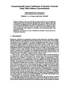
In this section, we present a computational soundness result for our abstraction of secure multi-party computations. Our result builds on the universal composability (UC) framework [25, 28], where the security of a protocol ρ is defined by comparison with an ideal functionality I. The proof proceeds in three steps, as depicted in Figure 3. In the first step, we prove that the robust safety of an applied π-calculus process carries over to the computational setting, where the protocol is executed by interactive Turing machines operating on bitstrings instead of symbolic terms and using cryptographic algorithms instead of constructors and destructors. This part of the proof solely depends on additional non-interactive cryptographic primitives that might be used in the protocol (such as encryption and digital signatures). It does not depend on the secure multi-party computations, which are still abstracted symbolically by processes of the form 3 The
source code can be found at http://www.lbs.cs.uni-saarland.de/publications/smpc_simap.spi. checked the protocol with 2 prices, 3 computation parties, and 2 input parties.
9
We type
Applied π calculus
Computational
Computational
Computational
execution
SMPC execution
SMPC execution
Ideal functionality I
Real SMPC ρ
Figure 3: Overview of the computational soundness proof SMPC(adv , sidc, in, F). Since the remaining steps of the proof are parametric over these non-interactive primitives, we decided to make our result general by assuming the first step of the proof, which is fairly standard and follows arguments similar to previous computational soundness results for non-interactive cryptographic primitives. In Appendix D, we prove the computational soundness of a specific Dolev-Yao model with asymmetric encryption, digital signatures, and arithmetic operations. The first part of the proof entails the computational soundness of a process executing the abstraction SMPC(adv , sidc, in, F). A computational implementation of the protocol, instead, should execute an actual SMPC protocol ρ. In the second step of the proof, we show that for each SMPC-suited context F, the computational execution of our abstraction SMPC(adv , sidc, in, F) is indistinguishable from the execution of a protocol I (see Construction 1) that solely comprises a single incorruptible machine. The third step of the proof builds on a result from [28], which ensures that for any well-formed ideal functionality I there is a protocol ρ that securely realizes I in the UC framework, which ensures in particular that the trace properties of I carry over to the actual implementation ρ. These three steps allow us to conclude that for each abstraction SMPC(adv , sidc, in, F) there exists an implementation ρ such that the trace properties of any well-formed process P (defined in Section 4.3), and in particular the security policies enforced by the type system, carry over from the execution that merely executes a process P and executes SMPC(adv , sidc, in, F) as a regular subprocess to the execution that communicates with ρ upon each call of a subprocess SMPC(adv , sidc, in, F). By leveraging the composability of the UC framework and the realization result for SMPC in the UC framework, we finally conclude that if a protocol based on our SMPC abstraction is robustly safe then there exists an implementation of that protocol that is computationally safe. We review the characterization of secure multi-party computations in the UC framework in Section 4.1. We present the computational execution for our SMPC abstraction in Section 4.2. In Section 4.3 we introduce the notion of computational safety. Finally, we state our computational soundness result in Section 4.4. Throughout the entire section, we use the notation that n is the number of parties in the current secure multi-party computation, i.e., for SMPC(adv , sidc, in, F) we have that n := |in|.
4.1
SMPC in the UC framework
UC Framework. The UC framework defines the security of a protocol ρ by comparison with an ideal functionality I. The ideal functionality for secure multi-party computations resembles our SMPC abstraction in that it essentially consists of a single machine performing an ideal computation. In the UC framework, a protocol ρ is called a secure realization of an ideal functionality I if for every attack on ρ there is an attack on I. More precisely, for any adversary that interacts with ρ, there is a simulator (often called the simulator)that interacts with I such that no protocol environment interacting with both the protocol and the adversary can tell an execution of ρ from an execution of I. In this work, all these 10
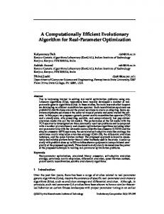
machines are polynomial-time. In the UC framework, a network is modelled as a set of interactive Turing machines (ITMs). Every ITM has a unique identity. The recipient of a message is addressed by the identity of that ITM. We say a network S is executable if it contains an ITM Z with distinguished input and output tape and with the special identity env. An execution of S with input z ∈ {0, 1} ∗ and security parameter k ∈ N is the following execution of the network: Initially, Z is activated with the message z on its input tape. Whenever an ITM M1 ∈ S finishes an activation with an outgoing message m (tagged with the identity of the receiver M2 ∈ S) on its outgoing communication tape, M2 is invoked with m (tagged with the identity of the sender M1 ) on its incoming communication tape. If an ITM terminates its activation without an outgoing message or sends a message to a non-existing ITM, the distinguished ITM Z is activated. The execution of the network terminates whenever Z writes a message on its distinguished output tape. A network S may also contain a distinguished ITM A, called the adversary. Sending a message over a public channel is modelled as sending a message to the adversary. A UC protocol is a network without an adversary and an environment. Corrupted parties are modelled as ITMs that directly forward all messages from and to the adversary. Moreover, the adversary can read all tapes of a corrupted party. In the UC framework, it is possible to model a port-based communication, i.e., each party has finitely many ports on which it can send (outgoing ports !p) or receive (incoming ports ?p) messages. In particular, in a session r every party i has an environment port ?inei,r , an environment port !outei,r , an adversary port ?inai,r , and an adversary port !outai,r . In all cases, port ?p is connected to some port !p and vice-versa. Hence, the incoming environment port ?inei,r and the outgoing environment port !outei,r are connected to an outgoing port !inei,r and an incoming port ?outei,r of the environment, respectively. Similar reasoning holds for the adversary ports ?inai,r , !inai,r , ?outai,r , and ?outai,r . As previously mentioned, in the UC framework the security of a protocol is determined by comparison with the ideal functionality. Intuitively, we say that a protocol ρ UC-realizes τ if there exists a simulator such that the interaction of ρ with the adversary and the interaction of τ with the simulator are indistinguishable. Definition 5 (Secure realization (UC) [25]). Let ρ and τ be protocols. We say that ρ UC-realizes τ if for any polynomial-time adversary A there exists a polynomial-time adversary S such that for any polynomial-time environment Z the networks ρ ∪ {A, Z} (called the real model) and τ ∪ {S, Z} (called the ideal model) are indistinguishable.4 SMPC in the UC framework. In Construction 1, we construct a generic ideal functionality Isid,F,c that serves as an abstraction of secure multi-party computations. This construction is parametric over the session identifier sid, the function F to be computed, and the corruption scenario c5 . This function is stateful, it expects the SMPC inputs and a state, and it outputs the result and an updated state. The ideal functionality receives the (secret) input message of party i from port ?inei,sid along with a session identifier. The input message is stored in the variable xi and the state state i of i is set to input. Both the session identifier and the length of the received message are leaked to the adversary, since in the actual implementation each party announces the session identifier and commits to its own private input, which leaks the length of that input (see part (a) of Construction 1). In addition, the (ideal) adversary is allowed to schedule the delivery of the results to party i, which is achieved by letting the adversary interact with the ideal functionality on port ?inai,sid (see part (b) of Construction 1). Since the ideal functionality might be reactive (i.e., the computation might involve different execution rounds), our construction additionally keeps a round counter for each participant i, denoted by ri . The construction is depicted in Figure 4. Construction 1 (SMPC Ideal functionality). We construct an interactive polynomial-time machine Isid,F , called the SMPC ideal functionality, which is parametric over a session identifier sid and a polytime algorithm F . Initially, the variables of Isid,F are instantiated as follows: ∀i ∈ [1, n].state i := input, ri := 1, and state F := ∅. Upon an activation with message m on port p, Isid,F behaves as follows. (a) Upon (?inei,sid , (m, sid0 )) If sid = sid0 and state i = input, then set state i := compute and xi := m. If state i = input, then send (sid0 , |m|) on port ?inai,sid . 4 Recall that the execution terminates whenever the environment writes on its output tape. We say that two executions E, E 0 are indistinguishable if |Pr[E = 1] − P r[E 0 = 1]| is negligible. 5 c = (c , . . . , c ) ∈ {0, 1}∗ where party i is corrupted if c = 1 and uncorrupted if c = 0. n 1 i i
11
?inei
(mi , sid� )
inputi
(|mi |, sid� )
!outai
store mi
check sid = sid�
computei ∀j : computej ?inai
(deliver, sid� )
run F (x1 , . . . , xn , state F ) (y1 , . . . , yn , s) ←
deliveri
!outei
Figure 4: The ideal functionality of SMPC (b) Upon (?inai,sid , (deliver, sid0 )), if ∀j ∈ [1, n].statej = compute and ri = rj , then compute (y1 , . . . , yn , s) ← F (x1 , . . . , xn , state F ) and set state F := s and ∀j ∈ [1, n].state j := deliver. If state i = deliver, set ri := ri + 1, state i := input and send yi on port !outei,sid . Since we consider static corruptions in this paper, the ports !outei,sid and ?inei,sid of the ideal functionality are redirected to the adversary whenever a party i is corrupted, as this party is under the control of the attacker. Such a port redirection is technically achieved by using dummy parties that act as message forwarders. We model the corruption scenario by a tuple c1 , . . . , cn of bits, where ci = 1 if and only if party i is corrupted. In the following, we denote by Isid,F,c the UC protocol composed of the ideal functionality Isid,F and the dummy parties required to connect the adversary to ports !outei,sid and ?inei,sid if ci = 1. The function F essentially plays the same role in the ideal functionality as the SMPC-suited context F in our symbolic abstraction of SMPC. In Section 4.2.1, we construct an algorithm FF for any F. Here, we only outline the construction: FF emulates F[deliver1 | . . . |delivern ] for a fixed reduction strategy. The inputs (x1 , . . . , xn ) of FF correspond to the messages that F receives over the local input channels lini ; the results of FF correspond to the messages sent by the context F[deliver1 | . . . | delivern ] on the output channels ini . Upon an empty input state stateF , FF emulates the process F[deliver1 | . . . | delivern ] and outputs a state s, which corresponds to the process that is left after the reduction has terminated. This state will be passed to the function in the next invocation, in order to deal with stateful computations. In this way, we are able to construct a family of ideal functionalities indexed by F instead of F . In the sequel, we refer to this ideal functionality as Isid,F ,c .
4.2
Computational execution of a process
Since the applied π-calculus only has semantics in the symbolic model (without probabilities and without the notion of a computational adversary), we need to introduce a notion of computational execution for applied π-calculus processes. Our computational implementation of a symbolic protocol P builds on the computational execution of the applied π-calculus that has been proposed in [8]. This is a probabilistic polynomial-time algorithm that expects as input the symbolic protocol Q, a set of deterministic polynomial-time algorithms A for the constructors and destructors in Q, and a security parameter k. This algorithm executes the protocol by interacting with a computational adversary. In the operational semantics of the applied π calculus, the reduction order is non-deterministic. This non-determinism is resolved by letting the adversary determine the order of the reduction steps. The computational execution sends the process to the adversary and expects a selection for the next reduction step. In the following,
12
we follow the convention that “fresh variable” or “fresh name” means a variable or name that does not occur in any of the variables maintained by the algorithm. The computational execution tightly follows the semantics of the applied π-calculus, with the exception that it operates on bitstrings and does not instantiate names and variables in the process but rather maintains an environment η that stores the bitstrings assigned to the free variables in P , and an interpretation µ of the free names in P as bitstrings. Given η and µ, we can computationally evaluate a term or a destructor application D to a bitstring cevalη,µ,k,A D by using the algorithms A for the constructors and destructors in D. (We will often omit k and A for readability if these are clear from the context.) We set cevalη,µ D := ⊥ if the application of one of the algorithms in A fails. In abuse of notation, in the following we will use evaluation contexts with distinguished multiple holes. The computational execution together with the adversary Advconstitutes a network. The adversary, however, can be seen as the environment; if the execution Execπ stops, Adv is activated. Definition 6 (Computational π-execution). Let Q be a closed process. Let C be an interactive machine called the adversary. We define the computational π-execution as an interactive machine ExecπQ,A (1k ) that takes a security parameter k as argument and interacts with C: • Start: Let P be obtained from Q by deterministic α-renaming so that all bound variables and names in Q are distinct. Let η and µ be a totally undefined partial functions from variables and names, respectively, to bitstrings. Let a1 , . . . , an denote the free names in P . For each i, pick ri ∈ Noncesk at random. Set µ := µ ∪ {a1 := r1 , . . . , an := rn }. Send (r1 , . . . , rn ) to C.6 • Main loop: Send P to the adversary and expect an evaluation context E from the adversary. Distinguish the following cases: – P = E[M (x).P1 ]: Request two bitstrings c, m from the adversary. If c = cevalη,µ M , set η := η ∪ {x := m} and P := E[P1 ]. – P = E[νa.P1 ]: Pick r ∈ Noncesk at random, set P := E[P1 ] and µ := µ(a := r). – P = E[M1 hN i.P1 ][M2 (x).P2 ]: If cevalη,µ M1 = cevalη,µ M2 , then set P := E[P1 ][P2 ] and η := η ∪ {x := cevalη,µ N }. – P = E[let x = D in P1 else P2 ]: If m := cevalη,µ D 6= ⊥, set η := η ∪ {x := m} and P := E[P1 ]; Otherwise set P := E[P2 ]. – P = E[assert F.P1 ]: Let P := E[P1 ] and raise the tuple ((F1 , . . . , Fn ), F, η, µ, P ) where assume F1 , . . ., assume Fn are the top level assumptions7 in P . – P˜ = E[!Q]: Let Q0 be obtained from Q by deterministic α-renaming so that all bound variables and names in Q0 are fresh. Set P := E[Q0 |!Q]. – P = E[M hN i.P1 ]: Request a bitstring c from the adversary. If c = cevalη,µ M , set P := E[P1 ] and send cevalη,µ N to the adversary. – In all other cases, do nothing. For any interactive machine Adv, we define ExecπQ,A,Adv (1k ) as the interaction between ExecπQ,A (1k ) and Adv; the output of ExecπQ,A,Adv (1k ) is the output of Adv. We let Assertions πP,A,p,Adv (k) denote the distribution of sequences of assertion tuples of the form ((F1 , . . . , Fn ), F, η, µ, P ) raised in an interaction of ExecπP,A,Adv (1k ) within the first p(k) computation steps (jointly counted for Adv(1k ) and ExecπP,A,τ (1k )). When applied to a protocol built on our abstraction of SMPC, the execution Execπ executes the abstraction SMPC(adv , sidc, in, F), which corresponds to a trusted host performing an ideal computation. Our computational soundness result, however, has to hold for an arbitrary protocol that incorporates an actual secure multi-party computation protocol. We thus introduce the notion of SMPC implementation Execsmpc , which differs from Execπ in that the SMPC protocol is executed instead of the abstraction SMPC(adv , sidc, in, F). Execsmpc takes as input the security parameter, a process Q, the algorithms A for the constructors and destructors in Q, and a family τ of UC protocols, one for each of the SMPC in Q. Intuitively, Execsmpc is meant to act as an interface between the adversary and the UC protocol, which can be either the ideal functionality or the actual SMPC protocol (i.e., τ will be either a family of ideal protocols or a family of real protocols, respectively). 6 In the applied π-calculus, free names occurring in the initial process represent nonces that are honestly chosen but known to the attacker. 7 assume F is top-level in P if there exists a context E such that P = E[assume F ].
13
ExecSMPC E[SMPC� (adv , in, F)] (i) E[c(z, s)][0r,in,F ] (ii)
Adv
�
0r,in,F SMPC(adv, sidc, in, F)
�
τr,F ,c
η(z := output i , E[c�x, s�][0r,in,F ] (iii)
s := r) !inei,r
E[0r,in,F ] (iv)
!inai,r
E[0r,in,F ] (v)
?outai,r i is corrupted store
?outei,r
?inei,r
?inai,r !outai,r !outei,r
outputi
Figure 5: The computational SMPC execution Execsmpc , sidc(sid).SMPC0 (adv , in, F) := SMPC(adv , sidc, in, F).
where
r
:=
µ(sid )
and
The behavior of Execsmpc is depicted in Figure 5, where sidc(sid).SMPC0 (adv , in, F) := SMPC(adv , sidc, in, F). The adversary may (i) initialize the secure multi-party computation, in which case a session identifier r is sent over the channel sidc; (ii) schedule the delivery of the output to some honest party, in which case the process and the environment η are updated accordingly; (iii) schedule the input of some honest party i, in which case this input is sent to the UC protocol over the port !inei,r ; (iv) schedule the input of some dishonest party i, in which case this input is sent to the UC protocol over the port connected to !inei,r ; and (v) send a message to party i, in which case this message is forwarded to port !inai,r . In all these cases, except for (i) and (ii), the computational execution interacts with the protocol and the protocol answers with a message m. If m is sent over the outgoing port of some honest party i (i.e., it is received from port ?outei,r ), then m is stored in a buffer waiting for delivery, otherwise m is directly forwarded to the attacker. The execution Execsmpc together with the adversary Adv and all the protocol parties for any session constitute a network. Each session r induces a subnetwork comprising the computational execution Execsmpc and the protocol parties for the session r. In this session r the execution Execsmpc plays the role of both the environment and the adversary, respectively, listening on the ports ?outei,r and ?outai,r (i ∈ [1, n]). In particular, Execsmpc is activated if no other machine in the subnetwork, composed of the is active anymore. If the execution Execsmpc terminates without having sent a message to a party, the adversary is activated. Definition 7 (Computational SMPC execution). Let Q and A be as in Definition 6. Let τ denote a family of UC protocols (intuitively, this family is composed of the implementations of the SMPC protocols for each of the SMPC-suited contexts F, the session identifiers r, and the corruption scenarios c, which k we denote by τr,F ,c ). We define the interactive machine Execsmpc Q,A,τ (1 ) by modifying the main loop of π k ExecQ,A (1 ) (see Definition 6) as follows: (i) (the secure multi-party computation is initialized) P = E[SMPC0 (adv , in, F)]. Set r := cevalη,µ (M ), η := η ∪ {sid := r}, and P := E[0r,in,F ].8 8 The SMPC abstraction is replaced by the dummy process 0 r,in,F , which is tagged with the session identifier r, the input channels in, and the function to be computed F .
14
(ii) (the output of some honest party is delivered) P = E[c(z, s).Q][0r,in,F ] and outputri = m 6= ⊥, and ∃i ∈ [1, n] : cevalη,µ ini = cevalη,µ c : Set η := η ∪ {z := m, s := r}, set outputri := ⊥, and P := E[Q][0r,in,F ]. (iii) (the input of some honest party is scheduled) P = E[chx, si.Q][0r,in,F ] and ∃i ∈ [1, n] : cevalη,µ ini = cevalη,µ c : Let m := cevalη,µ (x, s) and send m to τr,F ,c over the port !inei,r .9 (iv) (the input of some dishonest party is scheduled) P = E[0r,in,F ] Request a bitstring m from the adversary. If m = (ch, r, m0 ) and η(ini ) = ch for some i ∈ [1, n], send m0 over the port !inei,r . (v) (the adversary communicates with the protocol) P = E[0r,in,F ] Request a bitstring m from the adversary. If m = (i, r, m0 )10 then send m0 over the port !inai,r . In addition, in all cases but (i) and (ii), whenever a message m0 is received over a port ?outei,r with i not being corrupted, set outputri := m0 ; whenever a message m0 is received over ?outai,r or over ?outei,r for a corrupted i, (m0 , i) is forwarded to the adversary. Moreover, we do not send P to the adversary but the erasure of P in which all 0r,in,F are replaced by 0. k For any interactive machine Adv, we define Execsmpc Q,A,τ,Adv (1 ) as the interaction between smpc smpc k k ExecQ,A,τ (1 ) and Adv; the output of ExecQ,A,τ,Adv (1 ) is the output of Adv. We let Assertions smpc P,A,τ,p,Adv (k) denote the distribution of sequences of assertion tuples of the form k ((F1 , . . . , Fn ), F, η, µ, P ) raised in an interaction of Execsmpc P,A,τ,Adv (1 ) within the first p(k) computation smpc k k steps (jointly counted for Adv(1 ) and ExecP,A,τ (1 )). 4.2.1
The implementation of F
We construct for each F an algorithm FF that is computed by the ideal functionality Isid,F (see Construction 1). This algorithm emulates the computational π execution, i.e., FF additionally expects a state as input and outputs an updated state. For the construction of FF , we assume a fixed and efficiently computable reduction strategy S. This reduction strategy acts as the adversary, i.e., it constitutes an interactive machine (though in this construction the interaction as well as the interactive machines are emulated by FF ). Recall that the SMPC process contains internal loop channels inloop i for ensuring that every party only accepts a new input if an output has been delivered. The ideal functionality performs these checks directly; hence, we can omit these loop channels and we get (for n := |in|) F[in1 hy1 i | . . . | inn hyn i]. As F expects the inputs over the local input channels lin i , we place processes lini hxi i in parallel and set η(xi ) to be the ith input. Finally, in order to determine which message S schedules to be sent as an output, we place processes ini (yi0 , sid) in parallel and set the ith output to be ηˆ(yi0 ), where ηˆ is the variable mapping of the emulated execution after S finished. We assume an efficient encoding for processes and the name and variable mappings, µ and η. Let n := |in|; then, FF performs on input (m1 , . . . , mn , state) the following steps: 1. If state is empty, set compute state0 := F[in1 hy1 i | . . . | inn hyn i] and µ := η := ∅, where y 0 are fresh variables. Otherwise, try to extract a process P , a name mapping µ0 , and a variable mapping η 0 out of state. If this extraction fails abort; otherwise, set compute state0 := P, µ := µ0 , and η := η 0 . In both cases, with an empty state and a non-empty state, extend the variable mapping η ∪ {x1 := m1 , . . . , xn := mn } and set compute state := compute state0 | lin1 hx1 i | . . . | linn hxn i | in1 (y10 ) | . . . | inn (yn0 ).
2. Run the Main loop of the computational execution Execπcompute state,S with the name mapping µ and the variable mapping η. 9 !ine is connected to the incoming port ?ine i,r i,r 10 We implicitly assume that ∀i ∈ [1, n].µ(in ) ∈ i /
of party i in τr,F ,c [1, n].
15
3. Let compute state0 be the process to which compute state0 has been reduced after the reduction strategy S terminated. Let Let and ηˆ and µ ˆ be the variable and name mappings at that point. Let η (y10 ), . . . , ηˆ(yn0 ), state 0 ). If η(yi0 ) state 0 be the encoding of ηˆ, µ ˆ and compute state0 , and output (ˆ is undefined, output a distinguished error symbol.
4.3
Computational safety
For defining computational safety, we first need to recall the logic for the security policies that we are considering. The logic has to fulfill some standard properties such as monotonicity, closure under substitution, and it should allow the replacement of equals by equals. We assume a set Ds of deduction rules in the sequent calculus that define a deduction relation `s .11 Let Γ be a set of formulas in the logic. We say that a formula F is entailed by a premise Γ, denoted as Γ |=s F , if there is a proof tree (using Ds ) such that the conclusion of the deduction rule at the root of the tree is Γ `s F . Following the approach of Backes, Hritcu and Maffei [9], we characterize destructor application tests by introducing for each destructor an uninterpreted function symbol d# and a predicate Red such that Red(d# (M1 , . . . , Mn ), M ) holds true only if d(M1 , . . . , Mn ) = M holds true, where Mi , M are terms.12 We could assume Ds to contain the following deduction rule: d(M1 , . . . , Mn ) = M `s Red(d# (M1 , . . . , Mn ) = M
.
For the sake of a better presentation of the computational entailment relation, however, we want to keep the names of the variables that have been replaced by terms in the course of the execution. Therefore, we introduce a mapping eval from variables to terms that just stores which variable has been replaced by which term in the current process. Then, we represent the rule as d(eval(v1 ), . . . , eval(vn )) = M `s Red(d# (v1 , . . . , vn ) = v
,
with vi , v being variables only. Moreover, we assume Ds to contain rule for universal quantification: � 0� � 0� x x Γ `s C Γ, C `s B ,B x x L∀ x is free in Γ, C R∀ x is free in Γ, C, Γ, ∀x.C `s B Γ `s ∀x.C, B where x0 is a fresh variable. And, we assume analogous rules for existential quantification. The computational entailment relation |=η,µ,A is based on the symbolic entailment relation |=s . We define the computational entailment relation by the same inference rules with the only difference that universal quantification indeed quantifies over all bitstrings and all destructor application tests Red(d# (v1 , . . . , vn ), v) correspond to the check Ad (cevalη,µ v1 , . . . , cevalη,µ vn ) = cevalη,µ v, where Ad is the computational implementation of d. Definition 8 (Computational entailment |=η,µ,A ). Let `s be a symbolic entailment relation that is inductively defined by a set of inference rules Ds . Let η and µ be variable and name mappings, and let A be implementations. We define a set of inference rules Dη,µ,A as Ds with the following modifications: d(eval(v1 ), . . . , eval(vn )) = eval(v) `s d(v1 , . . . , vn ) = v Ad (cevalη,µ v1 , . . . , cevalη,µ vn ) = cevalη,µ v by , `η,µ,A d(v1 , . . . , vn ) = v
(a) Replace
11 We
refer the interested reader to [41]. The sequence calculus has been introduced by Gentzen in 1934 [40]. minor difference is that in our setting destructors are partial functions and in [9] destructors are defined via a reduction relation; in particular, destructors might be non-deterministic, i.e., relations. 12 One
16
�
� x0 Γ, C `s B x (b) replace x is free in Γ, C Γ, ∀x.C `s B � 0� x ∗ ∀b ∈ {0, 1} : Γ, C `η∪{x0 :=b},µ,A B x by x is free in Γ, C, and Γ, ∀x.C `η,µ,A B � 0� x Γ `s C ,B x (c) replace x is free in Γ, C Γ `s ∀x.C, B � 0� x ∗ ∀b ∈ {0, 1} : Γ `η∪{x0 :=b},µ,A C ,B x x is free in Γ, C, by Γ `η,µ,A ∀x.C, B
(d) replace all remaining `s by `η,µ,A .
We say that a formula F is entailed by a premise Γ, denoted as Γ |=η,µ,A F , if there is a proof tree (using Dη,µ,A ) such that the conclusion of the deduction rule at the root of the tree is Γ `η,µ,A F . We stress that we use the same computational entailment relation |=η,µ,A for both the computation πexecution and the computational SMPC-execution. The reason is that we consider first order formulas over free n-ary predicates and destructor application tests. There are properties for which computational soundness cannot be shown. For a function H whose range is smaller than its domain (such as a collision-resistant hash function), consider the injectivity property ∀x, y.x 6= y ⇒ H(x) 6= H(y). Symbolically, this property holds true if H is a constructor. Computationally, however, this formula naturally does not hold as x and y are universally quantified and collisions cannot be avoided. To exclude such cases, we only consider quantification over protocol messages. This is formalized by requiring that all quantified subformulas ∀x.F and ∃x.F are of the form ∀x.p(. . . , x, . . .) ⇒ F 0 and ∃x.p(. . . , x, . . .). ∧ F 0 (where p is a predicate) and we call the resulting class of first-order formulas well-formed formulas (seeDefinition 9). Hence ∀x, y.x 6= y ⇒ H(x) 6= H(y) is not well-formed. Instead, ∀x, y.p(x) ∧ p(y) ∧ x 6= y ⇒ H(x) 6= H(y)13 (where p is a predicate, meant to be assumed upon reception of x and y) is well-formed. As we exclude assumptions of the form ∀x.p(x), p(m) has to be assumed explicitly and m must be a protocol message. For a collision-resistant hash function H, the above formula holds computationally. We stress that in contrast to other computational soundness results (e.g., [8]), where formulas are assumed to be term-free (i.e., contain nullary predicates only), our result holds for formulas containing terms of the calculus and destructor application tests. Definition 9 (Well-formed formula). Let |=s be the entailment relation and Ds the set of deduction rules from above (the beginning of Section 4.3). Let x, x0 , xi denote variables, let p denote a predicate, and d a destructor. Let F be a formula over predicates p(x1 , . . . , xm ) and destructor application tests d(x1 , . . . , xm ) = x0 . We say that F is well-formed iff for all subformulas F 0 of F we have that • if F 0 = ∀x.F 00 , we have F 00 = p(. . . , x, . . . ) ⇒ F 000 (for some well-formed formula F 000 ), • if F 0 = ∃x.F 00 , we have F 00 = p(. . . , x, . . . ) ∧ F 000 (for some well-formed formula F 000 ). Such a p(. . . , x, . . .) is called the guard of x. A note on well-formed formulas. This well-formedness condition might seem heavily restrictive, but almost every formula can be easily converted into a well-formed formula. For example, the general security policy � ∀id, x, sid, z. ∧ni=1 Input(idi , xi , sid) ∧ id1 6= . . . 6= idn ∧ Frel ⇒ P(z, sid)
presented in Section 3 can be easily converted into a well-formed formula (given a free predicate p): n sid (sid) ∧ pmcp (z) ∀id, x, sid, z. ∧ni=1 pid i (id) ∧i=1 pi (x) ∧ p
� ∧ni=1 Input(idi , xi , sid) ∧ id1 6= . . . 6= idn ∧ Frel ⇒ P(z, sid).
13 This formula is logically equivalent to ∀x.p(x) ⇒ ∀y.p(y) ⇒ x 6= y ⇒ H(x) 6= H(y). For the sake of a clear presentation, the policies in Section 3 are not well-formed, but adding for every quantified variable x a predicate p(x) to the premise makes these policies well-formed as well.
17
This formula additionally requires that in the process at an appropriate place contains assume pa (m) for each pa (m) that occurs in the formula. For the computational soundness proof, we require all formulas to be well-formed. Moreover, in tight correspondence to the UC model, we require session identifiers to be unique. In addition, as we only consider static corruption, we need to require that the private channels ini (occurring in an SMPC occurrence SMPC(adv , sidc, in, F)) are never sent over a public channel. Hence, we require that a process only contains well-formed formulas and for all subprocess SMPC(adv , sidc, in, F) that the context F is SMPC-suited (see Definition 4), the channels ini are never sent over a public channel, every session identifier is sent at most once over a channel sidc. For the next definition, we need the following notation. We call a channel sidc that occurs in an SMPC subprocess SMPC(adv , sidc, in, F) process a session identifier channel and a channel ini that occurs in such an SMPC subprocess a party channel. A public channel is a channel that is either free or a channel that has been sent over a public channel. Definition 10 (Well-formed processes). A process P is well-formed if the following conditions hold: 1. For all asserts assert F in P the formula F is a predicate and for all assumes assume F the formula F is a well-formed formula. 2. For all subprocesses SMPC(adv , sidc, in, F) of P , F is an SMPC-suited context. 3. Every session identifier is only sent once over a session identifier channel sidc. 4. A non-free party channel ini (i.e., a term that contains ini ) is never sent over a public channel. We call a process an atomic process if it does not contain any assumptions and only assertions assert true and assert false. The computational notion of robust safety depends on the computational notion of logical entailment. We now introduce two definitions of robust computational safety, with respect to Execπ and Execsmpc , respectively. Definition 11 (Robust computational safety). Let P be a process, A an implementation of the destructors in P , and τ a family of secure multi-party computations. We say that P is π-(resp. SMPC-)robustly computationally safe using A (resp. A, τ ) iff for all polynomial-time interactive machines Adv and all polynomials p, Pr[for all ((F1 , . . . , Fn ), F, η, µ, Q) ∈ a, {F1 , . . . , Fn } |=η,µ,A F : a ← Assertions πP,A,p,Adv (k)]
(resp. Pr[for all ((F1 , . . . , Fn ), F, η, µ, Q) ∈ a, {F1 , . . . , Fn } |=η,µ,A F : a ← Assertions smpc P,A,τ,p,Adv (k)])
is overwhelming in k.
A symbolic model is computationally sound if robust safety carries over to the computational setting. This definition is used in our first theorem, which is parameterized over the non-interactive primitives used in the protocol. Definition 12 (Computationally sound model). Let A be a set of constructor and destructor implementations. We say that a symbolic model (D, P) is computationally sound using A iff for all P ∈ P such that P is robustly safe, P is π-robustly computationally safe using A. Definition 13 (Well-formed symbolic models). A symbolic model (D, P) is called well-formed if all processes P ∈ P are well-formed and P fulfills the following closure properties: (i) If P ∈ P and P 0 is a subprocesses of P , then P 0 ∈ P.
(ii) If P ∈ P, then νn.P ∈ P for any name n.
(iii) If P ∈ P and P 0 is statically equivalent to P , then P 0 ∈ P.
(iv) If P ∈ P and P 0 is an erasure of P obtained by replacing each assumption assume F with cp1 hv1 i | . . . cpn hvn i, where vi is a quantified variable with guards pi in F , and replacing each assert F 0 by cp01 (w1 ). . . . .cp0m (wm ).if d(v1 , . . . , vs ) = v then 0 else assert false where d ∈ D and w1 , . . . , wm are quantifies variables with guards p01 , . . . , p0m (respectively) that occur in an assume F 00 in P , then for this erasure P 0 we have νc. P, where c denotes all freshly introduced channels. 18
non–SMPC interaction
Adv
SSim ExecπP,A
SMPC
reschedule
interaction
Figure 6: The scheduling simulator SSim in interaction with the execution Execπ and the adversary. (v) If P ∈ P and P = P1 |P2 , then for Q := if d(M ) = N then assert false else 0|P2 we have Q ∈ P for any term M , N in the symbolic model and any destructor d ∈ D.
(vi) If P ∈ P and P = P1 |P2 , then for Q := if d(M ) = N then 0 else assert false|P2 we have Q ∈ P for any term M , N in the symbolic model and any destructor d ∈ D.
4.4
Computational soundness results
Finally, we are able to state our main results. In Section 4.4.1 we study the computational soundness of symbolic SMPC (Theorem 1), examining the main proof steps in Lemma 1, 2, 3, and 4. In Section 4.4.2 we present a computationally sound symbolic model with public-key encryption, digital signatures and arithmetic operations. 4.4.1
Computational soundness of symbolic SMPC
We now state the main computational soundness result of this work: the robust safety of a process using non-interactive primitives and our SMPC abstraction carries over to the computational setting, as long as the non-interactive primitives are computationally sound. This result ensures that the verification technique from Section 3 provides computational safety guarantees. We stress that the non-interactive primitives can be used both within the SMPC abstractions and within the surrounding protocol. Our proof of the next lemma utilizes that the simulator is able to compute the length of a message on its own. Therefore, we require of any implementation that the length of the output only depends on the length of the input. More formally, we say that a function f is length-regular, if for all x, y we have that |x| = |y| implies |f (x)| = |f (y)|. An algorithm A is length-regular if the function that A is length-regular, and a set A1 dots, An of algorithms is length-regular if every algorithm Ai , i ∈ [1, n], is length-regular. Lemma 1. For every well-formed atomic P , there exists a family I of SMPC ideal functionalities such that if P is π-robustly computationally safe using A and A is length-regular, then P is SMPC-robustly computationally safe using A, I. For brevity, we postpone the full proof to the appendix (see Appendix B) and only give a proof sketch at this point.
Proof sketch. We show that there is a ppt simulator SSim that we can plug in between Execπ and the adversary. Such that for any process well-formed process P , for any adversary Adv the interaction with the execution ExecπP,A together with SSim is indistinguishable from the interaction with the execution Execsmpc P,A,I (using the ideal functionality I) (see Figure 6). This simulator SSim simply forwards the messages as long as the messages do not belong to the interaction with an SMPC occurrence, i.e., as long as no subprocess SMPC(sidc, in, F) (for some sidc, in, and F) is scheduled by the adversary. For all messages in an interaction of an SMPC occurrence, SSim basically lets ExecπP,A behave like FF . In particular, SSim schedules the same reduction strategy S as FF (see Section 4.2.1). Moreover, in order to output the same leakage as I the scheduling simulator SSim needs to be able to compute the length of a message given the appropriate term. As all implementation algorithms are length-regular and the length of nonces is fixed, the scheduling simulator can efficiently compute the length of a message given the corresponding term. 19
We show that the two interactions, between ExecπP,A , SSim and Adv and between Execsmpc P.A,I and Adv, are indistinguishable for any Adv. Consequently, the statement follows. As a next step, we show that if a protocol ρ UC realizes our ideal functionality I, then, ρ is a sound implementation of SMPC as well. Lemma 2. Let ρ and I be two family of SMPC protocols and ideal functionalities such that ρ UC-realizes I (i.e., ρsid,F ,c ∈ ρ iff Isid,F ,c ∈ I and ρsid,F ,c UC realizes Isid,F ,c ). For every well-formed atomic P , if P is π-robustly computationally safe using A, I then P is SMPC-robustly computationally safe using A, ρ. For brevity, we postpone the full proof to the appendix (see Appendix C) and only give a proof sketch at this point. Proof sketch. We assumed ρ UC to realizes I; consequently, there is for any ppt adversary a ppt simulator such that for all environments the interaction between ρ and the adversary is indistinguishable from the interaction between I and the simulator. We only consider a dummy adversary that basically executes the commands of the environment. Moreover, for our setting, we instantiate the environments as (the emulation of) a pair of machines: the execution SMPC and a ppt machine that constitutes the adversary against SMPC, called hereafter the distinguisher. In Figure 7, P denotes the protocol, i.e., either ρ or F, respectively, Adv denotes the adversary, i.e., the ppt adversary Adv from the real setting or the simulator Sim, respectively. Moreover, the figures show the following connections (for a session r): • e denotes the connections between the environment output ports !outei,r and incoming ports of the environment ?outei,r and the environment input port !inei and outgoing ports ?inei,r of the protocol (for any i ∈ [1, |in|), • a denotes the connections between the adversary output ports !outai,r and incoming port ?outai,r of the adversary and the adversary input ?inai,r and outgoing ports !inai,r of the adversary, • ea denotes the connections between the output ports of the distinguisher A and input ports of the adversary for the distinguisher and the distinguisher A for the adversary, respectively, and finally • ea’ denotes the connections between the output ports of the execution and input ports of the adversary for the execution and the execution for the adversary, respectively. In the setting depicted in Figure 7, the UC protocol P directly communicates with the adversary Adv. The distinguisher can only communicate via the dummy adversary with the execution. The dummy adversary, forwards all messages of the form (i, s, m), where i ∈ [1, n] to the i party of the protocol session s; all other message are redirected to the execution. By assumption, the indistinguishability of the two interactions holds, i.e., between ρ and the dummy adversary and I and the simulator for the dummy adversary. As a next step, we transform the setting such that we are in the final setting. We modify the dummy adversary such that it redirects all messages to the execution (see Figure 8). We can show that in this setting the two interactions are indistinguishable as well i.e., the interaction between ρ and the dummy adversary and I and between the simulator for the dummy adversary. Consequently, the statement follows. It remains to show that there is are protocol that UC-realizes the ideal functionalities Isid,F ,c . In [28] a general construction is given for realizing any ideal functionality, which satisfies a particular wellformedness condition. Unfortunately, it turns out that their proof has a flaw. The problem with the construction is, basically, that their construction transforms any ideal functionality into a circuit, and all parties jointly compute this circuit. However, as they consider an attacker that controls the network, any potentially realizable ideal functionality has to hand the message delivery over to the ideal attacker. In particular the ideal functionality expects some message from the attacker for the message delivery. In the circuit that they construct, however, they close all input ports from the attacker. Hence, the circuit, which expects an order from the attacker for the message delivery, will not output anything. Therefore, as the ideal setting sends an output but he the realization does not, an environment can simply distinguish the two settings. We propose a simple fix: A well-formed ideal functionality, additionally, does not expect any message from the adversary. And we construct a wrapping machine W(τ ) that for a given well-formed ideal functionality τ and executes τ , leak the message lengths of the inputs, and sends the 20
e
A
P
Exec ea
A
Adv
ea�
Exec a
a
ea�
ea
e a
P
Adv Figure 7: The instantiation
Figure 8: The transformed setup
outputs upon a command from the ideal functionality. Then, we can apply the construction of [28] on the ideal functionality τ , yielding a protocol ρτ , and prove, along the lines of [28], that there is for any well-formed ideal functionality τ a protocol ρτ such that ρ UC realizes W(τ ). Our ideal functionality Isid,F ,c constitutes such an ideal functionality W(τ ), where τ is the submachine that executes F and stores the state of F . With these modifications, we are able to apply the result presented in [28]. Lemma 3. [28] Assume that enhanced trapdoor permutations exists. Then, for all Isid,F ,c there exists a non-trivial protocol in the CRS-model that UC realizes Isid,F ,c in the presence of malicious, static adversaries. We stress that Lemma 2, and therefore also Theorem 1, holds for any secure multi-party computation (SMPC) protocols that UC realizes our ideal functionality I. Other SMPC protocols might be attractive for efficiency reasons. However, other SMPC protocols might not realize the ideal functionality for any corruption scenario. Hence, they impose additional protocol constraints in that they require that for all occurrences SMPC(adv , sidc, in, F) only certain subsets of {in1 , . . . , inn } are free. As a next step, we show that computational soundness for atomic processes already suffices for guaranteeing computational soundness for the large class of well-formed processes. Lemma 4. Let (D, P) be a well-formed symbolic model. Assume there is an implementation A, ρ such that for all atomic processes P ∈ P the robust safety of P implies the SMPC-robust computational safety of P using A, ρ. Then also for all well-formed P ∈ P the robust safety of P implies the SMPC-robust computational safety of P using A, ρ. Proof. We prove the lemma by contradiction. First we assume that the initial process P is robustly safe but there is a set A of sequences of assertion tuples such that Pr[a0 ∈ A : a0 ← Assertions smpc P,A,τ,p,Adv )] is non-negligible and for all a ∈ A there is an assertion tuple t := ((F1 , . . . .Fn ), F, η, µ, Q) in a such that F1 , . . . .Fn 6|=η,µ,A F . Let for each such t (i.e., assertion tuple) Rt be a corresponding reduction sequence from the initial process P to the process Q with the variable and name mappings η and µ. In the applied π-calculus, we apply the reduction sequence Rt to the initial process P resulting in the same process Q (up to the renaming σ of the variables that has been performed by the computational execution). Claim 1: Rt is a valid reduction sequence. This claim follows from the computational soundness of atomic processes and by the subprocess closeness of P by induction over the reduction sequence. As P is robustly safe, we know that there is a proof tree T for the statement F |=s F over symbolic terms (see Definition 8). Let T 0 be the proof tree after replacing each occurrence of `s by `η,µ,A and each variable x that is free in the conclusion of the root of T by σ(x) (recall that σ is the renaming performed by the computational execution). We define a proof tree Tˆ based on T by applying the n o following replacements to T
replacement:
14
`s `η,µA
from the root to the leafs and by considering the fixpoint of this
14 We stress that this fixpoint exists because we have a tree structure. However, this fixpoint can be an infinite proof tree.
21
�
� η 0 ∪ {x0 := b} T T η0 ∗ � 0� � 0� ∀b ∈ {0, 1} : x x `η0 ,µ0 ,A B `η0 ∪{x0 :=b},µ0 ,A B Γ, C Γ, C x x (a) Replace by , Γ, ∀x.C `η0 ,µ0 ,A B Γ, ∀x.C `η0 ,µ0 ,A B �
� η 0 ∪ {x0 := b} T T η0 ∗ � 0� � 0� ∀b ∈ {0, 1} : x x Γ `η0 ,µ0 ,A C ,A Γ `η0 ∪{x0 :=b},µ0 ,A C ,A x x (b) replace by , Γ `η0 ,µ0 ,ulA ∀x.C, A Γ `η0 ,µ0 ,A ∀x.C, A (c) replace by
d(eval(v1 ), . . . , eval(vn )) = eval(v)
`η0 ,µ0 ,ulA Red(d# (v1 , . . . , vn ), v) Ad (cevalη0 ,µ0 v1 , . . . , cevalη0 ,µ0 vn ) = cevalη0 ,µ0 v `η0 ,µ0 ,A Red(d# (v1 , . . . , vn ), v)
, and finally
We claim that this (possibly infinite) tree Tˆ constitutes a proof tree for {F1 , . . . , Fn } |=η,µ,A F . Assume that there is a deduction step s that does not constitute a valid deduction step. As a tree is noetherian, we perform a noetherian induction over the proof tree. In the induction proof, we distinguish the following cases: � (i) (s is a ∀-rule) By induction T ab , is a proof tree and by construction s is valid. (ii) (s 6=
Ad (cevalη0 ,µ0 v1 , . . . , cevalη0 ,µ0 vn ) = cevalη0 ,µ0 v
and s is not a ∀-rule) In this case, there is a `η0 ,µ0 ,A Red(d# (v1 , . . . , vn ), v) already in T a corresponding step s0 that is invalid, which is a contradiction to the assumption that T is a valid proof tree. Ad (cevalη0 ,µ0 v1 , . . . , cevalη0 ,µ0 vn ) = cevalη0 ,µ0 v
) As all formulas are well-formed, each quan`η,µ,A Red(d# (v1 , . . . , vn ), v) tified variable in F are guarded. We say that a guard p(x) is necessary in F for F if and only if F |=s p(x), F |=s F , and for all F 0 such that F 0 6|=s p(x), we have F 0 6|=s F . As F |=s F we know that there is for each quantified variable x with a necessary guard p(x) an active assumption assume Fj such that Fj |=s p(x). We construct a process Pˆ out of the process P that is robust safe but not robust computationally safe. We introduce in Pˆ the restricted channel names cv , cv1 , . . . , cvn . As all formulas in the initial process P are well-formed, there is for each quantified vi an assumption assume Fj in Q that contains a predicate p that has vi as an argument, i.e., p(. . . , vi , . . . ). This assumption assume Fj also exists in the initial process P . Replace in P this assume Fj with cvi hvi i (analogously, for v). Then, we replace assert F with the following process:
(iii) (s =
cv (v).cv1 (v1 ). . . . .cvn (vn ).if d(v1 , . . . , vm ) = v then 0 else assert false Then, we erase all other assert and assume statements, i.e., replace them with 0. We observe that the resulting process νc. Pˆ , where c denotes all freshly introduced channels, is robustly safe as we assumed that P is robustly safe. By assumption, however, Pˆ is not SMPC-robustly computationally safe, which is a contradiction to the computational soundness of atomic processes.
We finally state our main computational soundness result. We apply a result of [28] for UC-realizable multi-party computation protocols for virtually all ideal functionalities. This result only holds under standard cryptographic assumptions. First, we assume that for each session all parties share a commonly known random bitstring, called the common reference string (CRS). Such a setup is called the CRS-model. 22
Second, we assume that enhanced trapdoor permutations exist, which roughly are permutations that are easy to compute and hard to invert unless a secret trapdoor is known. Moreover, as also required in other computational soundness results [15, 8], we require all implementations A to be length-regular (see Appendix B), i.e., the length of the output is easily computable by the length of the input (see Appendix B). Theorem 1 (Computational soundness of symbolic SMPC). Let (D, P) be computationally sound, wellformed model using A, where A is length-regular. If enhanced trapdoor permutations exist, then there is a family ρ of SMPC implementations in the CRS-model such that for each well-formed P ∈ P, the robust safety of P implies the SMPC-robust computational safety of P using A, ρ. Proof. The proof consists of four steps. Let atomic proceses be processes that only contain assertions of the form assert false and do not contain assumption. We show in Lemma 1 that for each atomic process P the π-robust computational safety using A implies SMPC-robust computational safety using A and I. In Lemma 2, we show for any two UC protocols τ and ρ such that τ UC-realizes τ 0 the SMPC-robust computational safety of P using A and τ 0 implies SMPC-robust computational safety using A and τ . If enhanced trapdoor permutations exist, we know by Lemma 3 that there is a protocol ρ that UC-realizes I in the CRS-model; hence, by applying Lemma 2 to ρ and I we obtain SMPC-robust computational safety using A and ρ for all atomic processes P . In Lemma 4 we show for each class of protocols P if the robust safety of each atomic P ∈ calP implies the SMPC-robust computational safety of P using A and ρ, then the robust safety of each well-formed P ∈ P also implies the SMPC-robust computational safety of P using A and ρ. 4.4.2
A computationally sound symbolic model with arithmetic operations
We show that our computational soundness result applies to a large class of protocols by proving the computational soundness of a symbolic model with public-key encryption, signatures, and arithmetics15 , including our case study with the sugar-beet double auction.We recall that numbers are modelled as symbolic bitstrings and arithmetic operations as destructors on these bitstrings. In this way, we enforce a strict separation between numbers and cryptographic terms, such as signatures and keys. Thus, it is not possible to apply an arithmetic operation on nonces, signatures, or encrypted messages. Due to this separation, the impossibility result for computational soundness of XOR [11] does not apply. As in [8], we impose some standard conditions on protocols to ensure that all encryptions and signatures are produced using fresh randomness and that secret keys are not sent around. A protocol satisfying these conditions is called key-safe. We denote the resulting symbolic model as (DESA , PESA ). The computational soundness proof for (DESA , PESA ) follows almost exactly the lines of the symbolic model for key-safe protocols in the work of Backes, Hofheinz, and Unruh [8]. Therefore, we postponed the proof to the appendix (Appendix D). Theorem 2 (Computational soundness of (DESA , PESA )). If enhanced trapdoor permutations exist, there is an length-regular implementation A such that (DESA , PESA ) is a computationally sound, well-formed model. As a corollary of Theorem 1 and Theorem 2, we get the computational soundness of protocols using SMPC, public-key encryption, signatures, and arithmetics, with such non-interactive cryptographic primitives possibly used within both SMPC and the surrounding protocol. Corollary 1 (SMPC computational soundness with (DESA , PESA )). There is an implementation A and a family of UC-protocols τ such that for each well-formed P ∈ PESA , the robust safety of P implies the SMPC-robust computational safety of P using A and τ .
5
Conclusion
We have presented an abstraction of SMPC in the applied π-calculus. We have shown that the security of protocols based on this abstraction can be automatically verified using a type system, and we have established computational soundness results for this abstraction including SMPC that involve arbirtrary 15 This
result extends prior work [8] in the CoSP framework to arithmetics and first-order logic formulas.
23
arithmetic operations. This is the first work to tackle the abstraction, verification, and computational soundness of protocols based on an interactive cryptographic primitive. Our framework allows for the verification of protocols incorporating SMPC as a building block. In particular, the type-checker ensures that the inputs provided by the participants to the SMPC are wellformed and, after verifying the correctness of SMPC, the type-checker obtains a characterization of the outputs (e.g., in the Millionaires problem, the output is the identity of the participant providing the greatest input) that can be used to establish global properties of the overall protocol. Our framework is general and covers SMPC based on arithmetic operations as well as on cryptographic primitives. This work focuses on trace properties, which include authenticity, integrity, authorization policies, and weak secrecy (i.e., the attacker cannot compute a certain value)16 . As a future work, we plan to extend our framework to observational equivalence relations, possibly building on recent results for a fragment of the applied π-calculus [30]. It would be interesting to formulate and verify an indistinguishabilitybased secrecy property for SMPC. This task is particularly challenging since the result of an SMPC typically reveals some information about the secret inputs and standard secrecy definitions based on observational equivalence are thus too restrictive. An additional problem is the computational soundness of observational equivalence for processes with private channels, which are excluded in [30] but are needed in our abstraction and, arguably, in any reasonable SMPC abstraction.
5.1
Future work
Generalizing computational soundness for interactive primitives for arbitrary calculi We proved our abstraction computationally sound with respect to the applied π calculus. The CoSP framework (see Appendix D) of Backes, Hofheinz, and Unruh [8] provides a general model for proving non-interactive primitives to be a computationally sound abstraction with respect to a large class of calculi (including the applied π calculus or RCF[19]). An interesting direction for future research is the extension of the CoSP framework to interactive primitives. Characterizing arithmetic functions with a computationally sound implementation Showing computationally soundness for arithmetic functions is known to be troublesome and even impossible for group operations in most Dolev-Yao models, as shown by Backes and Pfitzmann [11].17 However, for many applications, such as auction protocols or voting schemes, arithmetic functions are unavoidable; hence, it would be interesting to characterize the class of arithmetic functions that are Dolev-Yao abstractable in a computationally sound way. Computational soundness for arbitrary functionalities Although it is possible to model virtually any interactive primitive with our abstraction, such as zeroknowledge proof systems, the resulting implementation is not allowed to leak more than the message length and would therefore be far more inefficient than, e.g., a usual zero-knowledge proof system. More specifically, our abstraction does not allow functionalities in which the ideal adversary sends or receives messages directly to or from the functionality. Many efficient protocols are realizations of functionalities that have more leakage than only the message length or allow the adversary to have more influence than merely to decide which messages are delivered. With our proof method it is possible to show computational soundness for protocols that emulate these functionalities as well, assuming there is a protocol that UC realizes such a functionality. We believe that is suffices to incorporate the additional leakage and the additional influence capabilities of the adversary into SMPC (see Figure 1) and the general ideal functionality (see Construction 1) and to adjust the scheduling simulator (see Appendix B) to the modified process SMPC. We believe that, then, it is possible to show that the modification of SMPC is a computationally sound abstraction of such a more efficient protocol. 16 To symbolically model weak secrecy, one can add the process c(x).if x=n then assert false (where c is a public channel) to check the secrecy of n: The protocol is robustly safe only if the attacker does not learn n. 17 Actually, only the impossibility result for XOR has been shown, yet the same reasoning applies to any group operation.
24
Special-purpose implementations Our result considers at the moment a general secure multi-party computation (SMPC). For generality, we disallow assumptions and assertions to be placed inside the SMPC abstraction. An implementation, however, that is tailored to our computational execution Execsmpc would allow for placing assumptions and assertions inside our SMPC abstraction while staying computationally sound. Such an implementation would extend the verification possibilities. Acknowledgements. We thank Dominique Unruh for numerous insightful discussions about simulation based security and computational soundness. Moreover, we thank Fabienne Eigner and Kim Pecina for their intensive support on the case study. We are also grateful for the helpful comments of the anonymous reviewers.
25
Appendix A
Postponed definitions
A.1
The syntax and semantics of the applied π-calculus M, N ::=
terms
x, y, z
variables
a, b, c
names
f (M1 , . . . , Mn )
constructor application
D ::=
destructor term
M
terms
d(M1 , . . . , Mn )
destructor application
P, Q ::=
processes
M hN i.P
output
M (x).P
input
0
nil
P |Q
parallel composition
!P
replication
νa.P
restriction
let x = D
let
in P else Q
P |0≡P P ≡Q
assume F
assumption
assert F
assertion
P ≡P
Q≡R
P ≡R
νa.νb.P ≡ νb.νa.P
(P | Q) | R ≡ P | (Q | R) P ≡Q
a∈ / fn(P )
P |R≡Q|R
νa.(P | Q) ≡ P | νa.Q
N ≈ N0
d(M ) = N 6= ⊥
N hM i.Q | N (x).P → Q | P {M/x}
let x = d(M ) in P else Q → P {N/x}
P ≡Q νa.P ≡ νa.Q
P |Q≡Q|P
0
d(M ) = ⊥ let x = d(M ) in P else Q → Q
let x = N in P else Q → P {N/x}
P →Q P |R→Q|R
P →Q P0 ≡ P
Q ≡ Q0
P →Q 0
νa.P → νa.Q
P →Q P |R→Q|R
P0 ≡ P
0
P →Q P 0 → Q0
νa.P → νa.Q
26
!P → P | !P
Q ≡ Q0
B
From the π-execution to the SMPC-execution
In this section, we present the proof of Lemma 1. Lemma 1.For every well-formed P , there exists a family I of SMPC ideal functionalities such that if P is π-robustly computationally safe using A, then P is SMPC-robustly computationally safe using A, I. Let an occurrence of a subprocess SMPC(adv , sidc, in, F) in a process P be called an SMPC session. Recall that the SMPC execution Execsmpc for every SMPC session SMPC(adv , sidc, in, F) does not reduce the subprocess SMPC(adv , sidc, in, F) itself but interacts with a UC protocol, which we call the implementation of SMPC. The lemma states that there is a family of ideal functionalities in interaction such that for all well-formed processes P all valid assertions in the computational execution Execπ with an implementation A also hold in the computational execution Execsmpc with an implementation A and I (as an implementation of SMPC). The family of ideal functionalities I is constructed in Construction 1. The proof compares the computational execution Execπ with the computational execution Execsmpc that uses the ideal functionality I as the implementation of SMPC. More precisely, let k be the security parameter and p be an arbitrary polynomial; we show that there is a polynomially bounded function l and a machine SSim, called the scheduling simulator, such that for all well-formed processes P , all implementations A, and all adversaries Adv we have that the distribution Assertions πP,A,(p+l),hSSim,Advi (k) is statistically indistinguishable from the distribution Assertions smpc P,A,I,p,Adv (k) for all k.
B.1
The construction of the scheduling simulator
The scheduling simulator SSim basically schedules the reduction steps that correspond to the action of I. SSim simulates against an adversary Adv the execution Execsmpc while interacting withExecπ . We stress that SSim does not have additional capabilities compared to a usual adversary against Execπ . As SSim does not know the bitstring η(sid) corresponding to the symbolic session identifier sid from the beginning of the execution, SSim internally assigns an identifier γ to every SMPC occurrence SMPC(adv , sidc, in, F) and tags in an internal copy of the current process SMPC(adv , sidc, in, F) (and later on 0r,in,F ) with γ, denoted as SMPC(adv , sidc, in, F)γ and 0r,in,F as 0r,in,F ,γ .18 There is a discrepancy between the process that is executed by Execπ and the process that the adversary expects from the simulation of Execsmpc : In Execsmpc every SMPC session is replaced by 0r,in,F after initialization; in Execπ , on the other hand, every SMPC session is treated as a regular subprocess. Therefore, for each SMPC(adv , sidc, in, F) occurrence γ, the scheduling simulator stores the state of this occurrence in a process smpc state(γ). Moreover, SSim stores the current process for the adversary as P˜ and keeps track of the modifications as follows. SSim translates the evaluation context from the adversary by replacing every SMPC(adv , sidc, in, F)γ (or 0r,in,F ,γ , respectively) by ˆ to address the subprocess smpc state(γ). Thereafter, SSim uses the translated evaluation context E π to be reduced in the execution Exec and sends appropriate evaluation contexts until the process in Execπ is a desired state. At this point SSim updates P˜ such that it corresponds to a reduction step in the execution Execsmpc . The process smpc state(γ) consists of a subprocess compute state(γ) for the current state of F and a context smpc frame(γ)[•], i.e., smpc state(γ) := smpc frame(γ)[compute state(γ)]. smpc frame(γ)[•] can be characterized by the state of every party. Therefore, SSim maintains a function state π with which SSim keeps track of the state state π (γ, i) of a party i in an SMPC session γ. In Definition 14, we formally define the context smpc frame(γ)[•]. There is a yet another gap between I and SMPC: The ideal functionality I expects an explicit command (i, s, deliver) for outputting the result; on the other hand, the process SMPC(adv , sidc, in, F) expects an appropriate sequence of evaluation contexts. Moreover, we need to maintain two partial mappings sessionid and µ ˜. sessionid (γ) is in the course of the execution assigned the real session identifier as soon as the upon receiving the first accepted input, the real session identifier is leaked to the adversary. 18 Similar
to the computational execution, SSim does not send 0r,in,F ,γ to the adversary but only 0.
27
This mapping is used to later on check, whether the adversary addresses the commands to the correct session. µ ˜ stores the all channel bitstrings that the execution Execπ sends to the adversary, such as the bitstrings for the private channels of the corrupted parties. In some cases, SSim checks whether for a given term c there is an i such that cevalη,µ ini = cevalη,µ c. Although SSim does not know η and µ, the simulator can efficiently perform this check as it knows all intermediate processes and, hence, all reduction steps. Characterizing the state of an SMPC session. For the construction of SSim we need to characterize the different states of the distinguished process SMPC(adv , sidc, in, F). This is done by a context, called smpc frame(γ)[•], that is defined in Definition 14. In our abstraction, every party of a secure multiparty computation can be in the following states: init, input, compute, and deliver. In the state init, the entire session is not initialized yet; in the state input, the party expects an input; in the state compute, the party is ready to start the main computation; and, in the state deliver, the party is ready to deliver a message. These states are stored in a mapping state π (which is maintained by SSim) such that state π (γ, i) is the state of party i in the session γ. Definition 14 (smpc frame). Let a mapping state π from internal session identifiers and party identifiers to states given. We assign a process to each state stateπ (γ, i). Let α := (state π , γ, (adv, sidc, in, F)). state π (γ, i) = input : inpi (α) = ini (xi , sid0 ).advhsid0 i. if sid = sid0 then lini hxi i else inloopi hsync()i | inputi 4 state π (γ, i) = compute : inpi (α) = lin1 hxi i | inputi 4 state π (γ, i) ∈ {deliver, init} : inpi (α) = inputi 4
We define the context initp(α) as initp(α)[•] = sidc(sid).νlin. νinloop.(•) if for all i ∈ [1, |in|] 4
state π (γ, i) = init and initp(α)[•] = • otherwise. We define the context smpc frame(γ)[α] as follows. 4
smpc frame(α)[•] = 4
� � initp(α) inp1 (α) | . . . | inpn (α) | •
In the construction of SSim, state π and (adv, sidc, in, F) are mostly clear from the context; more precisely, in the construction state π is globally defined and for every γ there is only one tuple (adv, sidc, in, F). Hence, if there is no ambiguity we also write smpc frame(γ)[•] for smpc frame(α)[•]. The scheduling simulator keeps track of subprocesses Q in a process P ; this is done via a context E such that E[Q] = P . As the process P might be reduced, we need for every reduction step of the process an appropriate reduction step of the context E. Definition 15 (Reduction of a context). Let P be a process, Q be a subprocess, and E be the evaluation context such that E[Q] = P . We say that P is reduced to P 0 if there is a subprocess R of P and a corresponding evaluation context L such that L[R] = P and there is a process R0 such that P 0 = L[R0 ]. We say that the evaluation context E is reduced to E 0 according to the reduction from P to P 0 if there is a context L0 with two distinct holes such that L0 [R][Q] = P , L0 [R][•] = E[•], and L0 [•][Q] = L[•] and L0 [R0 ][Q] = P 0 and L0 [R0 ][•] = E 0 [•]. Construction of SSim. Before we present the actual construction of the scheduling simulator, we introduce some notation for convenience. Throughout this section we use n for the amount of parties in an SMPC occurrence, i.e., for an occurrence SMPC(adv , sidc, in, F) we consider n to be |in|. With abuse of notation, we denote the replacement of every occurrence of 0r,in,F ,γ in a process P by smpc state(γ) as � � smpc state(γ) P . 0r,in,F ,γ Analogously, we write for an evaluation context E for the context in which each occurrence of 0r,in,F ,γ is replaced by smpc state(γ) as � � smpc state(γ) E . 0r,in,F ,γ 28
o n ˜ and a process P˜ the abbreviations E ˆ := E ˜ smpc state(γ) , Pˆ := We use for a context E 0r,in,F ,γ o n smpc state(γ) 0 ˜ , and sidc(sid).SMPC (adv , in, F) := SMPC(adv , sidc, in, F). P 0r,in,F ,γ
1. Upon receiving the initial process P0 , set P˜ := P0 . Enumerate every occurrence SMPC(adv , sidc, in, F) with an internal session identifier γ, and tag this occurrence SMPC(adv , sidc, in, F) in P˜ with γ. Let initially for each γ compute state(γ) := F, delivery(γ, i) := f alse, let sessionid(γ) be completely undefined, and let state π (γ, i) := init for all i ∈ [1, n]. For any γ let corrupt(γ, i) := true, if the corresponding ini in SMPC(adv , sidc, in, F) is free; otherwise let corrupt(γ, i) := false. Forward all bitstrings that are initially sent by the execution Execπ to the adversary. In addition store all channel names in the partial mapping µ ˜. Then proceed as in 2. 2. Main loop: Let P be the last process that has been sent by the execution Execπ . Check whether Pˆ = P . If the check fails, stop the entire simulation. Otherwise, construct the erasure of P˜ , i.e., remove in P˜ the tag γ from each SMPC(adv , sidc, in, F) and remove the tag (r, in, F, γ) from ˜ each 0r,in,F ,γ . Send the erasure of P˜ to the adversary Adv. Then, expect an evaluation context E. ˜ We distinguish the following cases for E. ˜ schedules the initialization (a) E 0 ˜ • Evaluation context: P˜ = E[SMPC (adv , in, F)γ ] • State check: Check whether state π (γ, i) := init for all i ∈ [1, n]. Schedule appropriate reduction steps until the current process in Execπ is ˆ E[smpc frame(state 0π , γ, α)[compute state(γ)]], where α := (adv, sidc, in, F) and state 0π (γ, i) := input for all i ∈ [1, n] and state 0π coincides with state π on all other arguments.19 ˜ r,in,F ,γ ], stateπ (γ, i) := input for all i ∈ [1, n]. Set P˜ := E[0
˜ schedules an input to a corrupted party i. (b) E ˜ r,in,F ,γ ] • Evaluation context: P˜ = E[0 • State check: Request a bitstring m from the adversary. Check whether m = (c, s, input, m0 ) and stateπ (γ, i) = input. Schedule appropriate reduction steps until the current process in Execπ is ˆ E[smpc frame(state 0π , γ, α)[compute state(γ)]],
where α := (adv, sidc, in, F) and state 0π (γ, i) := compute and state 0π coincides with state π on all other arguments. In the first reduction step, the execution Execπ requests a message and the bitstring for the channel ini . Upon such a request of the execution, send (c, (m0 , s)) in response. If the execution does not accept the channel name c, i.e., if c 6= µ(ini ), we schedule appropriate reduction steps until the current process of Execπ is again ˆ E[smpc frame(state π , γ, α)[compute state(γ)]]. Moreover, in that case we leave P˜ and state π (γ, i) unchanged. If the execution accepts the channel name c, we proceed and check in case µ ˜(ini ) is defined whether c = µ ˜(ini ); if µ ˜(ini ) is not defined set µ ˜(ini ) := c. If the check fails, abort the entire simulation. Set channel (γ, i) := c. Execπ requests in a later step the bitstring µ(adv) for the channel adv. Upon such a request, send cadv and expect a bitstring s0 in response. Forward (s0 , |m0 |, i) to the adversary and store the session identifier s0 that is sent to the adversary upon an accepted input, i.e., set sessionid (γ) := s0 . Reduce for all j 6= i for which context(γ, i) is defined context(γ, j) according to the reduction steps that have just been scheduled. Set stateπ (γ, i) := compute, and let P˜ remain unchanged. 19 Recall
that we have at this point compute state(γ) = F [deliver1 | . . . | delivern ], as the session has just been
initialized.
29
˜ schedules an input to an honest party i. (c) E ˜ • Evaluation context: P˜ = E[chx, si.Q][0r,in,F ,γ ]
• State check: Check whether there is an i ∈ [1, n] such that cevalη,µ c = cevalη,µ ini , stateπ (γ, i) = input, and delivery(γ, i) = false. n o state(γ 0 ) Let Q0 := Q smpc . Schedule appropriate reduction steps until the current process 0r,in,F ,γ of Execπ is ˆ E[smpc frame(state 0π , γ, α)[compute state(γ)]],
where α := (adv, sidc, in, F) and state 0π (γ, i) := compute and state 0π coincides with state π on all other arguments. Execπ requests in a later step the bitstring µ(adv) for the channel adv. Upon such a request, send cadv and expect a bitstring s0 in response. Recall that all implementations are lengthregular; as we know the length of the nonces, we can compute the message length of any message. Let xi be the input term for party i. We compute the length of the bitstring η(xi ) corresponding to the input of party i. Then, we send (s0 , l, i) to the adversary and store the session identifier s0 that is sent to the adversary upon an accepted input, i.e., set sessionid (γ) := s0 . Reduce for all j 6= i for which context(γ, i) is defined context(γ, j) according to the reduction steps that have just been scheduled. ˜ Set stateπ (γ, i) := compute, and P˜ := E[Q][0 r,in,F ,γ ]. (d) Start the main computation upon the first delivery command for a party i. ˜ r,in,F ,γ ] • Evaluation context: P˜ = E[0
• State check: Request a bitstring m from the adversary. Check whether s = sessionid (γ) and stateπ (γ, i) = compute for all i ∈ [1, n]. Moreover, check whether (i) m = (i, s, deliver) or (ii) m = (c, s, deliver). In case (ii), check furthermore whether there is an i ∈ [1, n] such that c = µ ˜(ini ).
Simulate the execution Execπ on the process
Q := compute state(γ) | lin1 hx1 i | . . . | linn hxn i | in1 (y10 , sid) | . . . | inn (yn0 , sid) | {z } | {z } =:Qlin
=:Qin
against the fixed and efficiently computable reduction strategy S that is used by FF (see Section 4.2.1) as follows: – (an input is read ) For every context E[•1 ][•2 ] = E 0 [•1 ] | E 00 [•2 ] | Qin that is sent by S such that E 00 [P 0 ][lini hxi i] = Qlin for some P 0 , send E 000 [•1 ][•2 ]
ˆ := E[inp 1 (α) | . . . | inpi−1 (α) | •2
| inputi | inpi+1 (α) | . . . | inpn (α) | E 0 [•1 ]]
to the execution Execπ , where α := (state π , γ, (adv, sidc, in, F)) and inpj (α) is defined as ˆ in Definition 14. Receive an updated process P 0 =: E[smpc frame(γ)[compute state(γ)]] 0 from the execution. If P is unmodified (i.e., P 0 = E 000 [P 0 ][lini hxi i]]), send compute state(γ) | Qlin | Qin as a response to E to the reduction strategy S. Otherwise if P 0 = E 000 [P 00 ][0]], send E 0 [P 00 ] | E 00 [0] | Qin as a response to E to the reduction strategy S. Update Qlin := E 00 [0] and reduce for all i for which context(γ, i) is defined the context context(γ, i) according to the reduction of compute state(γ) (see Definition 15). In all other cases, abort the entire simulation of SSim. – (a step inside F is performed ) For every context E[•] = E 0 [•] | Qlin | Qin that ˆ is sent by S, send E[smpc frame(γ)[E[•]]] to the execution. Receive the updated 0 ˆ process P =: E[smpc frame(γ)[compute state(γ)]] from the execution and send compute state(γ) | Qlin | Qin as a response to E to the reduction strategy S. Reduce for all i for which context(γ, i) is defined the context context(γ, i) according to the reduction of compute state(γ) (see Definition 15). Do the same for an evaluation context E with two distinct holes, i.e., for E[•1 ][•2 ] = E 0 [•1 ][•2 ] | Qlin | Qin . 30
– (an output is sent) For every context E[•1 ][•2 ] = E 0 [•1 ] | Qlin | E 00 [•2 ] that is sent by S such that E 00 [ini (xi )] = Qin and compute state(γ) = E 0 [deliveri ], store context(γ, i) := E 0 [•]. Send E 0 [0] | Qlin | E 00 [0] as a response to E to the reduction strategy S. Update Qin := E 00 [0] and reduce for all i for which context(γ, i) is defined the context context(γ, i) according to the reduction of compute state(γ) (see Definition 15). Let P 00 be the last process that has been sent by Execπ . Set stateπ (γ, i) := deliver for ˆ frame(γ)[compute state(γ)]] := all i ∈ [1, n]. Update compute state(γ), i.e., set E[smpc P 00 . Let P˜ remain unchanged. Thereafter, proceed as in the case of a delivery command for corrupted parties (case 2e). (e) The delivery command for a party i is sent. ˜ r,in,F ,γ ] • Evaluation context: P˜ = E[0 • State check: Request a bitstring m from the adversary. Check whether s = sessionid (γ), and stateπ (γ, i) = deliver and either (i) m = (i, s, deliver) or (ii) m = (c, s, deliver). In case (ii) additionally check whether there is an i ∈ [1, n] such that µ ˜(ini ) = c. In case (i), set delivery(γ, i) := true, state π (γ, i) = input, and let P˜ remain unchanged. In case (ii), schedule appropriate reduction steps until the current process of Execπ is ˆ frame(state 0π , γ, α)[context(γ, i)[0]]], E[smpc where α := (adv, sidc, in, F) and state 0π (γ, i) := input and state 0π (γ 0 , j) := state π (γ 0 , j) for all (γ 0 , j) 6= (γ, i). Upon a request from the execution Execπ for a bitstring, send µ ˜(ini ) to Execπ . Ex0 0 0 pect a pair (m , s ) and forward (m , i) to the adversary. Reduce for all j 6= i for which context(γ, i) is defined context(γ, j) according to the reduction steps induced by ˆ E[smpc frame(γ)[context(γ, i)[•]]]. ˆ state(γ)] := P 0 . Let P˜ Let P 0 be the last process that has been sent by Execπ . Set E[smpc remain unchanged. Set stateπ (γ, i) := input. (f) The output of party i is delivered to an honest party. ˜ • Evaluation context: P˜ = E[c(x).Q][0 r,in,F ,γ ]
• State check: Check whether there is an i such that cevalη,µ c = cevalη,µ outi . Check whether stateπ (γ, i) = input, delivery(γ, i) = true. n o state(γ 0 ) Let Q0 := Q smpc . In case (ii), schedule appropriate reduction steps until the 0r,in,F ,γ π current process of Exec is ˆ 0 ][smpc frame(state 0π , γ, α)[context(γ, i)[0]]], E[Q
where α := (adv, sidc, in, F) and state 0π (γ, i) := input and state 0π (γ 0 , j) := state π (γ 0 , j) for all (γ 0 , j) 6= (γ, i). Reduce for all j 6= i for which context(γ, i) is defined context(γ, j) according to the reduction ˆ steps induced by E[smpc frame(γ)[context(γ, i)[•]]]. 0 ˜ Let P be the last process that has been sent by Execπ . Set P˜ := E[Q][0 r,in,F ,γ ] and delivery(γ, i) := false. (g) P˜ = E[!Q]: For each bound variable and name in Q, choose fresh variables, or name, from the same equivalence class, according to the same enumerations as in Execπ , yielding a process Q0 . For any SMPC(adv , sidc, in, F) occurrence in Q, assign a fresh internal identifier γ and set for all i ∈ [1, n] state π (γ, i) = init, compute state(γ) := F, delivery(γ, i) := false, corrupt(γ, i) := true if ini is free in the initial process P0 , and corrupt(γ, i) := false otherwise. smpc state(γ) ˜ /0r,in,F ,γ }. If the check Check whether the process in response is equal to E[Q]{ 0 ˜ fails, abort; otherwise, set P := E[E[Q | !Q]. ˜ (x).Q]: Request two bitstrings (c, m) from the adversary. Send to the execution E. ˆ (h) P˜ = E[M π If Exec requests two bitstrings, we send (c, m). Check whether the process in response is smpc state(γ) ˜ equal to E[Q]{ /0r,in,F ,γ }. If the check fails, abort; otherwise, set P˜ := E[Q]. 31
˜ hN i.Q]: Request a bitstring c from the adversary. Send to the execution E. ˆ If the (i) P˜ = E[M execution requests a bitstrings send c and expect a bitstring m. Check whether the term N is actually a channel c. If the check succeeds, set µ ˜(c) := m. Send m to the adversary Adv. smpc state(γ) ˜ /0r,in,F ,γ }. If Moreover, check whether the process in response is equal to E[Q]{ ˜ the check fails, abort; otherwise, set P := E[Q]. ˜ ˆ and check whether the process in response is equal to (j) P˜ = E[νa.Q]: Send to the execution E. smpc state(γ) ˜ E[Q]{ /0r,in,F ,γ }. If the check fails, abort; otherwise, set P˜ := E[Q].
ˆ and check whether the process in ˜ 1 hN i.P1 ][M2 (x).P2 ]: Send to the execution E. (k) P˜ = E[M smpc state(γ) ˜ response is equal to E[Q]{ /0r,in,F ,γ }. If the check fails, abort; otherwise, set ˜ 1 ][P2 ]. P˜ := E[P ˜ ˆ and check whether the process (l) P˜ = E[let x = D in P1 else P2 ]: Send to the execution E 00 smpc state(γ) ˜ /0r,in,F ,γ } with P 00 ∈ {P1 , P2 }. If the check fails, in response is equal to E[P ]{ 00 abort; otherwise, set P˜ := E[P ] with the matching P 00 . ˜ ˆ and check whether the process in response is (m) P˜ = E[assert(F ).Q]: Send to the execution E smpc state(γ) ˜ equal to E[Q]{ /0r,in,F ,γ }. If the check fails, abort; otherwise, set P˜ := E[Q]. (n) In all other cases do nothing.
A note on the network model. Recall that every time a party A sends a message to a party B, the machine B is activated. Hence, upon activation by the execution, i.e., when SSim receives a process or a message from Execπ , or by the adversary, i.e., when SSim receives an evaluation context or a message from Adv, it might happen that SSim first finishes his actions from the previous round and only thereafter reads the new input from the execution.
B.2
The proof of the soundness of SSim
The proof compares the parts of the internal state of ExecπP,A,hSSim,Advi with parts of the internal state of Execsmpc P,A,I,Adv , which is shown in Lemma 5. The proof proceeds by induction over the evaluation contexts that Adv has sent. The sequence of internal states that is being compared is defined in Definition 16. We perform an induction over the internal states of the two settings. However, there are slight technical mismatches between the two settings. These mismatches are not essential to the proof and are removed in Definition 16where we define the two distributions over the (adjusted) internal states. In Lemma 5, we show that these two distributions are statistically indistinguishable. Notation. For an SMPC occurrence smpc state(γ), we need for each i ∈ n the notion of the input and the output variable of party i. Recall the process inp i from the smpc frame (see Definition 14): inp i = Q|inputi . If there is a subprocess lini hxi i in Q, then xi is called the input variable of smpc state(γ). The output variable of party i in smpc state(γ) is defined via context(γ, i). If context(γ, i) is defined and smpc frame(γ)[context(γ, i)[deliveri ]] = smpc state(γ), then yi in ini hyi , sidi.inloopi hsync()i is called the output variable of party i in smpc state(γ). Let ⊥ be a distinguished error symbol. Moreover, for the sequence of internal states, we enumerate all SMPC occurrences in Execsmpc P,A,I,Adv with internal session identifiers γ in the same way as the scheduling simulator SSim. Definition 16 (Internal states). Let P be a process. Let Adv be a machine, called the adversary. Let Execsmpc be as in Definition 7, and Execπ be as in Definition 6. The rth round of Execsmpc P,A,I,Adv is the rth round of the main loop of Execsmpc . The rth round of ExecπP,A,hSSim,Advi is the rth round of the main loop of SSim. • (m0r , n0r , mr , nr ) Let m0r be the messages that are sent in ExecπP,A,hSSim,Advi to the adversary Adv in the rth round and n0r be the messages that are sent by the adversary Adv in the rth round; analogous with mr and nr for Execsmpc P,A,I,Adv .
32
γ,r γ,r := xi from the ideal functionality Iu,in,F ,γ (see Construction 1).20 • (result γ,r i , input i ) Let input i γ,r Analogously, let result i := yi from the ideal functionality Iu,in,F ,γ . On the other hand, for and yiγ,r be the input and output variable, respectively, of party i in ExecπP,A,hSSim,Advi let xγ,r i smpc state(γ) in round r.
• (compute state) Let compute stateγr be the process that FF would extract from stateF . If γ 0γ γ stateF = ∅ set compute 0 := F [0]. On the other hand, let compute stater be the process � deliverstate i of SSim, i.e., for every i every occurrence of a process deliveri is compute state(γ) 0 replaced by the empty process 0. • (η 00 , µ00 ) η 00 and µ00 are the variable and name mapping of Execπ restricted on all variables and names, respectively, that are not locally bounded in a subprocess smpc state. η and µ are the variable and name mapping, respectively, of Execsmpc . • (ηγ , µγ ) Let Iγ denote the session in Execsmpc that belongs to the internal session identifier γ. The variable and name mappings ηγ and µγ are the mappings that FF in Iγ would extract from stateF . The mappings ηγ0 and µ0γ are obtained by restricting η 0 and µ0 to the variables and names, respectively, in smpc state(γ). • (state 0π ) Let state 00π be the state mapping of SSim in round r. Then, let state 0π (γ, i) := ⊥ if state 00π (γ, i) = init and state 0π (γ, i) := state 00π (γ, i) otherwise. On the other hand, in Execsmpc , let Iγ denote the session that belongs to the internal session identifier γ. Let state π (γ, ·) be the state mapping of Iγ . If I has not been initialized yet, set state π (γ, i) := ⊥ for all i ∈ [1, n]. Let Γ(r) be the set of all internal session identifiers in round r. Let ((ms , ns ), (compute stateγs )γ∈Γ(r) , statesπ , (η s , µs ), (inputγ,s )γ∈Γ(r) , (resultγ,s )γ∈Γ(r) )rs=0 be the sequence of internal states of the execution Execsmpc P,A,I,Adv up to the rth round. Let s
s
s
0 00 00 0 γ,s ((m0s , n0s ), (compute state0γ ))γ∈Γ(r) , (η 0 (y γ,s ))γ∈Γ(r) )rs=0 s )γ∈Γ(r) , stateπ , (η , µ ), (η (x
be the sequence of internal states of the execution ExecπP,A,I,hSSim,Advi up to the rth round. Adv Let TP,r be the distribution of the rth extended prefix of the execution Execsmpc P,A,I,Adv and, analoAdv
gously, T 0 P,r be the distribution for ExecπP,A,hSSim,Advi For proving Lemma 1, we show that for all security parameters k and for all polynomials p there is a polynomially bounded function l and a machine SSim such that for all well-formed processes P , all implementations A, and all adversaries Adv we have that the distribution Assertions πP,A,(p+l),hSSim,Advi (k) is statistically indistinguishable from the distribution Assertions smpc P,A,I,p,Adv (k). For proving the indistinguishability of these two distributions over assertion tuples, we show an even stronger property: We show that even the distributions over the sequences of internal states of both settings are statistically indistinguishable. Lemma 5is shown by an induction over the internal states of the two settings. D
D Lemma 5. Let TP,r and T 0 P,r be defined as in Definition 16). Then, for all machines D and for all r ∈ N D D the two distributions TP,r and T 0 P,r are statistically indistinguishable, i.e., for all (possibly unbounded) interactive machines D, all polynomials p, and all r ∈ N there is a k0 ∈ N such that for all k > k0 h i � � k 0D D Pr b = 1 : b ← D(1k , t), t ← TP,r − Pr b = 1 : b ← D(1 , t), t ← T P,r ≤ p(k)
holds true.
Proof. We prove the statement by induction on the round r of Main loop, of either the execution Execsmpc or the scheduling simulator SSim. More precisely, our induction hypothesis is that the two distributions D D TP,r−1 and T 0 P,r−1 are indistinguishable for any distinguisher D. The processes that are sent to the adversary are indistinguishable as long as all checks on expect in SSim succeed. 20 In
particular, input γ,r := ⊥, if xi is undefined. i
33
For r = 0, we only need to compare Start. In Start both Execsmpc and Execπ only send the free names and the initial process to the adversary. Moreover, the initially the current process is the same in both settings, and we have for all γ γ compute stateγ0 = compute state0γ 0 = F [0].
Hence, T0 and T00 are indistinguishable. For r > 0, we assume that Tr−1 and T 0 r−1 are statistically indistinguishable. Hence, all previously sent subprocesses are indistinguishable in both settings. As we can see by the construction of SSim, Execsmpc , and Execπ , in all cases the check P = P˜ succeeds. Let P be the process that has been sent to the adversary at the beginning of round r. ˜ that is sent by the adversary in We distinguish the following cases for the evaluation context E smpc ˜ response to the last process P that has been sent by SSim or Exec , respectively. Recall that stateπ is maintained by I as well as by SSim. With abuse of notation, we denote both state π and state 0π from Tr and Tr0 , respectively, with the mapping state π in the following case distinction. ˜ schedules the initialization. (a) E 0 ˜ • Evaluation context: P˜ = E[SMPC (adv , in, F)γ ]
• State: state π (γ, i) := ⊥ for all i ∈ [1, n]
The scheduling simulator SSim sets state0π (γ, i) := input for all i ∈ [1, n]. On the other hand, initially, the internal state of Ir,F is set to input. No other values in Tr and Tr0 change compared to the round r − 1; hence and by induction hypothesis, Tr and Tr0 are indistinguishable.
˜ schedules an input of a corrupted party i. (b) E ˜ r,in,F ,γ ] • Evaluation context: P˜ = E[0
• State: A bitstring m has been requested from the adversary. (c, s, input, m0 ), s = sessionid (γ), and stateπ (γ, i) = input.
Check whether m =
The scheduling simulator first sends evaluation contexts such that the execution asks for a channel 0 name c, a message m0 , and a session id s for ini (xγ,r i , sid), and, then, the simulator sends (c, (s, m )). In the two settings the probability that c = cevalη,µ ini and sid = cevalη,µ sidγ is the same, where η and µ denote the variable and the name mapping of Execsmpc or Execπ , respectively. If the two 0 bitstrings are accepted, we have η(xγ,p i ) = m . On the other hand, we know by the construction of I 0 that inputpi = m0 holds true as well. By the induction hypothesis we know that Tr−1 and Tr−1 are computationally indistinguishable. As only the list of inputs differs r − 1 and r and we have seen π that Execsmpc P,A accepts the inputs with the same probability as ExecP,A,SSim accepts the input, Tr 0 and Tr are computationally indistinguishable. ˜ schedules an input for an honest party i. (c) E ˜ • Evaluation context: P˜ = E[chx, si.Q][0r,in,F ,γ ]
• State: There is an i ∈ [1, n] such that cevalη,µ c = cevalη,µ ini and stateπ (γ, i) = input. By construction of the computational ideal functionality, the computational ideal functionality accepts if and only if SMPC accepts the input. Moreover, we know that inputγ,r = η(xγ,r i i ) and 0 stateπ (γ, i) = compute. By induction hypothesis, we conclude that Tr and Tr are indistinguishable. (d) Start the main computation before delivering the first result for party i. ˜ r,in,F ,γ ] or (ii) P˜ = E[c(x).Q][0 ˜ • Evaluation context: (i) P˜ = E[0 r,in,F ,γ ]
• State: A bitstring m has been requested from the adversary. stateπ (γ, i) = compute for all i ∈ [1, n]. Moreover, either (i) m = (c, s, deliver) and s = sessionid (γ) or (i) m = (i, s, deliver0 ) and s = sessionid (γ). In case (ii), check additionally whether there is an i ∈ [1, |ini |] such that cevalη,µ c = cevalη,µ ini .
34
At this point there is a mismatch between the two settings: If in Execsmpc P,A,I,Adv the adversary sends a delivery request for a party that is uncorrupted party and for which the channel name has not been already sent to the adversary, there is an exponentially small chance of the adversary succeeding; in the communication with the scheduling simulator, on the other hand, there is no chance of succeeding. However, this situation only happens with exponentially small probability. As a first step, let us note that by Definition 4f v(F[0]) ⊆ ∅. η(f v(F[0])) is contained in Tr−1 and 0 η 0 (f v(F[0])) is contained in Tr−1 . Hence, by induction hypothesis, η(f v(compute state(γ))) and 0 0 η (f v(compute state (γ))) are indistinguishable. I as well as SSim runs the main computation whenever deliver is scheduled and state π (γ, i) = compute for all i ∈ [1, n] where in are the channels involved in the session γ. Recall that I and SSim use the same reduction strategy and that this reduction strategy schedules the same reduction steps. r−1 r−1 , By induction hypothesis, we know that state r−1 , µγr−1 , compute stateγr−1 and state 0π π , ηγ γ r−1 r−1 η 0 γ , µ0 γ , compute state0 r−1 are indistinguishable.21 γ,r Since SSim as well as FF run Execπcompute state(γ),A , FF (inputγ,r 1 , . . . , inputn , stateF ) =: γ,r (resultr1 , . . . , resultrn ) and η 0 (y1 ), . . . , η 0 (ynγ,r ) are indistinguishable for a distinguisher that is given 0 Tr−1 or Tr−1 Moreover, as compute stater−1 = compute state0r−1 holds by induction hypothesis, compute stater = compute state0r .
Thereafter, we are in the case for delivery with corrupted parties or honest parties, respectively. (e) The delivery command for a party i is sent. ˜ r,in,F ,γ ] • Evaluation context: P˜ = E[0
• State: A bitstrings m has been requested from the adversary, stateπ (γ, i) = deliver, and (i) m = (i, s, deliver) and s = sessionid (γ) or (ii) m = (c, s, deliver) and s = sessionid (γ). In case (i), we set in both settings state π (γ, i) to input. Hence, Tr and Tr0 remain indistinguishable. In case (ii), in both settings the bitstring c is sent to the execution. If c = η(ini ) the result is sent to the adversary in both settings. Moreover, both settings set state π (γ, i) := input. By induction hypothesis, or as we have already seen in the case (d), we know that these two results are computationally indistinguishable. Hence, we conclude that Tr and Tr0 are indistinguishable. (f ) The output of party i is delivered to an honest party. ˜ • Evaluation context: P˜ = E[c(x).Q][0 r,in,F ,γ ]
• State: There is an i such that cevalη,µ c = cevalη,µ ini and stateπ (γ, i) = input. We stress that the scheduling simulator can compute whether there is an i such that cevalη,µ c = cevalη,µ ini . We have the invariant that delivery(γ, i) = true if and only if outputi is defined. Hence, both ExecπP,A,hSSim,Di and Execsmpc P,A,I,D perform a message synchronization, i.e., the message is output to the honest party. r
r
By induction hypothesis resultγ,r−1 and µ(yiγ,r ) are indistinguishable; hence, η r , µr and η 00 , µ00 are i indistinguishable as well. Therefore, Tr and Tr0 are indistinguishable as well. (g) In all other cases, either the scheduling simulator only replaces the unreduced SMPC with the ˜ and forwards the modified evaluation current state smpc state of Execπ in the evaluation context E context to Execπ , or both SSim and either Execsmpc or I ignore the evaluation context. Since Execπ coincides on these cases with Execsmpc and the scheduling simulator only forwards messages, Tr and Tr0 are indistinguishable as well.
21 Formally,
r−1 D we consider the distribution obtained by projecting TP,r−1 and T 0 D , ηγr−1 , µr−1 , γ P,r−1 to (state π
, µ0 γr−1 , compute state0 γr−1 ), respectively. compute stateγr−1 ) and (state 0π r−1 , η 0 r−1 γ
35
Finally, we prove the lemma. Lemma 1. For every well-formed P , there exists a family I of SMPC ideal functionalities such that if P is π-robustly computationally safe using A, then P is SMPC-robustly computationally safe using A, I. Proof of Lemma 1. In Lemma 5we show that the distributions over the sequence of processes that are sent to the adversary are indistinguishable. Hence, it suffices to solely show that the messages inside the events are indistinguishable. But, as the two executions coincide on all processes that do not contain D SMPC, assertion tuples that contain message that are distinguishable can be used to distinguish TP,r D from T 0 P,r which, however, is a contradiction to Lemma 5.
C
Leveraging UC-realizability
In this section, we show that the notion of UC-realization implies the SMPC-robust computational safety (see Definition 11) in our framework. Lemma 2.[Leveraging UC-realizability] Let ρ and I be two family of SMPC protocols and ideal functionalities such that ρ UC-realizes I (i.e., ρsid,F ,c ∈ ρ iff Isid,F ,c ∈ I and ρsid,F ,c UC realizes Isid,F ,c ). For every well-formed P , if P is π-robustly computationally safe using A, I then P is SMPCrobustly computationally safe using A, ρ. Proof. Let A be a set of constructor and destructor implementations. Then, we show that for all processes Q in the applied π calculus and for all ppt machines Adv, hereafter called the distinguisher, there is a ppt machine Sim such that for all ppt machines A the following indistinguishability holds true for A the two smpc distributions are indistinguishable Execsmpc Q,I,ρ,hAdv,Ai and ExecQ,I,I,hSim,Ai . This indistinguishability, in turn, implies that h i Pr ((F1 , . . . , Fn ), F, η, µ) ∈ Assertions smpc Q,A,I,p,hSim,Ai (k), {F1 , . . . , Fn } |=η,µ,A F i h (k), {F , . . . , F } |= F − Pr ((F1 , . . . , Fn ), F, η, µ) ∈ Assertions smpc 1 n η,µ,A Q,A,ρ,p,hAdv,Ai is negligible. Hence, the statement follows. The proof begins with the UC setting. As ρ UC realizes I, we know that for all ppt adversaries M there is a simulator Sim such that for all ppt environments E the following two settings are indistinguishable: first, P := ρsid,in,F and Adv := M and, second, P := Isid,in,F and Adv := Sim. By the universal UC
composability [25] and as assumed ρ ≥ F , we know that for any polynomial p p(k)
X i=1
UC
ρi ≥
p(k)
X i=1
Ii
holds true where ρi + ρj denotes the concurrent execution of ρi and ρj and k is the security parameter. Consequently, there is a simulator for the concurrent execution of all sessions. Throughout the proof, we denote by Sim that simulator. The figures show, for clarity, only the transformations on one protocol session, but we perform the transformations on all sessions simultaneously. As the UC realization property ensures that for all adversaries there is a valid simulator for all environment, we can concentrate on one particular adversary and a subset of all possible environments. In the course of the proof, we basically consider the dummy adversary, called MD . Moreover, we split the environment E into two parts. The first part constitutes a ppt distinguisher A, and the second part constitutes the computational execution Execsmpc Q,A . Then, we transform the environment E in several steps in which the messages from the distinguisher A and the UC adversary Adv are redirected such that after each transformation the two settings remain indistinguishable for A. In Figure 9 and Figure 10, P denotes the protocol, i.e., either ρ or F, respectively, Adv denotes the adversary, i.e., the ppt adversary Adv from the real setting or the simulator Sim, respectively. Moreover, the figures show the following connections (for a session r): 36
e
A
P
Exec ea
A
Adv
ea�
Exec a
a
ea�
ea
e a
P
Adv Figure 9: The instantiation
Figure 10: The transformed setup
• e denotes the connections between the environment output ports !outei,r and incoming ports of the environment ?outei,r and the environment input port !inei,r and outgoing ports ?inei,r of the protocol (for any i ∈ [1, |in|), • a denotes the connections between the adversary output ports !outai,r and incoming port ?outai,r of the adversary and the adversary input ?inai,r and outgoing ports !inai,r of the adversary, • ea denotes the connections between the output ports of the distinguisher A and input ports of the adversary for the distinguisher and the distinguisher A for the adversary, respectively, and finally • ea’ denotes the connections between the output ports of the execution and input ports of the adversary for the execution and the execution for the adversary, respectively. The instantiation (Figure 9): We consider a family of environments that consist of two parts: a ppt distinguisher A and the computational SMPC execution Execsmpc Q,A . The distinguisher A can only communicate with the execution Execsmpc and the UC adversary Adv. The execution is modified in that Q,A all messages (i, s, m), which the execution would usually send over an adversary port to the protocol, are ignored. Recall that we have a nested scheduling order: Whenever a protocol party of the UC attacker is stops without sending a message, the execution is activated. Whenever the execution stops the distinguisher is activated.22 We restrict our attention to the UC adversary, hereafter called MD , that basically executes the commands of the adversary. As we consider static corruption, the dummy adversary only needs to forward messages. Upon a message m, MD checks whether m = (i, sid, m0 ) and i ∈ [1, |in|], where sid is the session identifier of every party.23 If the check succeeds, MD sends m0 over the port !inai . Otherwise, send m over ea0 . As ρ UC-realizes F, there is a simulator Sim for each ppt adversary such that the two settings are indistinguishable for all environments E(A, Execsmpc Q,A ) where A is an arbitrary ppt machine. The transformed setup (Figure 10): We change the setting such that all ports from the protocol that have been connected to the adversary ports (a) are here connected to the environment. Analogously, all ports from the adversary (a) that have been connected to the protocol are here connected to the environment. In particular, all corrupted parties do not redirect the messages to the UC adversary Adv 0 anymore but send the messages to the execution. Here, we consider the machine MD that internally runs 0 0 MD and forwards everything to MD . Whenever MD wants to send a message m over !inai,r , MD sends 0 0 0 m := (i, sid, m ) to the execution. As MD reverts the effect of MD , effectively MD only forwards every message from the distinguisher A. We do the same transformation for the simulator SimMD obtaining a simulator Sim0MD . Moreover, we consider usual execution Execsmpc Q,A . In particular, the execution forwards all messages 0 that it receives over a port ?outai,r to the UC adversary MD . And, for every message (i, s, m) that is received by the adversary, the execution forwards m over !inai,r . We stress that the execution does not pay attention over which port a message has been sent by the adversary; the execution processes all of them in the same way. After these modification we effectively are in the situation in which A only communicates with the adversary, the adversary only communicates with the execution, and the execution communicates with 22 Technically,
these two machines are emulated by one master-machine that respects the constraints mentioned. that we assumed that the channel names are distinct from [1, n] for the maximal number of parties in Q that perform a joint secure multi-party computation. 23 Recall
37
the adversary and the protocol. The execution checks upon a message over a channel ?outei whether i is corrupted. If the check succeeds, the execution forwards the message to the adversary. Hence, the execution only forwards the messages that are addressed to the adversary. Two settings, consequently, remain indistinguishable for A. More precisely, given a successful distinguisher for the two settings in this transformed setup, we can construct a successful distinguisher for the initial setup, which contradicts assumption that ρi UC realizes Ii . 0 As MD merely forwards every message, we have shown that for any ppt distinguisher A the following smpc . two settings are indistinguishable: Execsmpc 0 ,Ai and ExecQ,A,A ,hSim0 Q,A,Aρ ,hMD I MD ,Ai It remains to show that the following difference is negligible: h i Pr ((F1 , . . . , Fn ), F, η, µ) ∈ Assertions smpc (k), {F , . . . , F } |= F 1 n η,µ,A Q,A,I,p,hSim,Ai h i . − Pr ((F1 , . . . , Fn ), F, η, µ) ∈ Assertions smpc (k), {F , . . . , F } |= F 1 n η,µ,A Q,A,ρ,p,hAdv,Ai The assumption tuples that are raised can only differ in the messages that they contain, since the process is observable to the distinguisher. The two executions, however, only differ in the implementation of SMPC; hence, it remains to show that the messages sent over e are indistinguishable. Above, we showed that by the UC security, we can conclude that the messages that are sent over e are indistinguishable in the two settings (see Figure 9). As the execution is a polynomial-time machine, everything it computes out of indistinguishable inputs remains indistinguishable. Hence, the statement follows.
D
Computational soundness of key-safe protocols with arithmetics
In this section, we first show how to leverage computational soundness proofs from CoSP to our framework (Section D.1). We translate from the variant of the applied π-calculus that is presented in this work to the variant of the applied π-calculus in [8], which has been proven in [8] to inherit computational soundness results from CoSP. Then, we review the CoSP framework (Section D.2), introduce a symbolic model for public-key encryption, signatures, and arithmetic operations (Section D.3), present the implementation conditions for the computational soundness result (Section D.4), extending the symbolic model and the implementation conditions for public-key encryption and signatures presented in [8], and finally we present the computational soundness proof for the presented symbolic model (Section D.5). With minor modifications the computational soundness proof in [8] for public-key encryption and signatures directly applies to the extended model; in the proof we highlight the modifications in bold.
D.1
Translating processes
The applied π calculus considered in [8] is a variant of the calculus that we consider in the current work. Instead of assumes and asserts they only provide atomic events, i.e., events that do not carry a message. Security properties are expressed as properties over traces of atomic events. The operations semantics of their variant of the applied π calculus comprises an additional rule for reducing events, and each reduction step may be labelled by an event. With this notation, a process is said to satisfy a property if for every reduction sequence the sequence of raised events is in the trace property. The computational execution of the applied π calculus with events, presented in [8], is basically identical to Execπ with the difference that a sequence of events is output instead of a sequence of assertion tuples. A process is said to computationally satisfy a trace property if for any adversary the probability that the event trace is in the trace property (in a polynomially long interaction) is overwhelming. We introduce two notions: first, the applied π calculus with atomic events representing the calculus that is used in [8], and, second, the applied π calculus with assumes and asserts representing the calculus that is used in the present work. The translation. We simply erase in a process P all occurrences of assert true and replace all occurrences of assert false with event bad, obtaining a process T (P ). The trace property Tp (P ) then simply requires that the event bad has not been raised. Then, the following lemma follows immediately. 38
Lemma 6. There is a translation T from processes to processes and a translation Tp from processes to traces such that the following holds true: For any well-formed process P (in the applied π calculus with assumes and asserts) if P is robustly safe, then, T (P ) satisifies Tp (P ). Moreover, whenever T (P ) computationally satisfies Tp (P ), P is robustly computationally safe. Proof. There is a strong correspondence between P and T (P ) as the operational semantics of the two calculi almost coincide. The only difference is that in the applied π-calculus with asserts and assumes asserts are not reduce, while in the calculus with atomic events the events are reduced. We have the following property: Let P be an atomic process in the applied π-calculus with asserts and assumes. After applying an arbitrary reduction sequence to T (P ), i.e., T (P ) →∗ P˜ we distinguish two cases. Either the event bad has been raised in P˜ . In this case, there is reduction sequence such that P →∗ P 0 , P˜ = T (P 00 ), P 00 is a subprocess of P 0 (modulo associativity and commutativity), and there is a top-level assume false in P 0 . Or no event bad has been raised and there is a reduction sequence such that P →∗ P 0 and P˜ = T (P 0 ). The lemma directly follows from this observation. Before we present the modified proof from the work of Backes, Hofheinz, and Unruh [8], we present the proof of our second main theorem. Theorem 2.[Computational soundness of (DESA , PESA )] If enhanced trapdoor permutations exist, there is an length-regular implementation A such that (DESA , PESA ) is a computationally sound, well-formed model. Proof. By Lemma 6, we know that if an atomic process (in the applied π-calculus with assumes and asserts) P is robustly safe, then the trace property (see Definition 23) Tp (P ) for the process T (P ) holds true. In [8] it has been shown that there is an embedding from the applied π-calculus with atomic events into CoSP protocols (see Definition 17) such that trace properties are preserved. In Lemma 12, we show that the symbolic model presented in Section D.3 is computationally sound. In [8], a computational πexecution is presented upon which Execπ is based. Moreover, Backes, Hofheinz, and Unruh show in [8] that trace properties a preserved from the computational (CoSP-)execution and their computational π-execution. The translation function from CoSP protocols to processes, presented in [8], also preserves containment in the image of T . Moreover, we consider the closure of the resulting symbolic model under the conditions in Definition 13 is well-formed. Hence, with Lemma 6, we can conclude the proof.
D.2
Review of CoSP
Backes, Hofheinz, and Unruh presented a framework for conducting computational soundness proofs [8]. This framework separates the task of proving computational soundness for a set of (non-interactive) primitives against Dolev-Yao attackers from the task of embedding a calculus into a setting with a symbolic Dolev-Yao attacker. We give an overview of the ideas underlying CoSP. All definitions in CoSP are relative to a symbolic model that specifies a set of constructors and destructors that symbolically represent computational operations, and a computational implementation that specifies cryptographic algorithms for these constructors and destructors. In CoSP, a protocol is represented by an infinite tree that describes the protocol as a labeled transition system. Such a CoSP protocol contains actions for performing abstract computations (applying constructors and destructors to messages) and for communicating with an adversary. A CoSP protocol is endowed with two semantics, a symbolic execution and a computational execution. In the symbolic execution, messages are represented by terms. In the computational execution, messages are bitstrings, and the computational implementation is used instead of applying constructors and destructors. A computational implementation is computationally sound if any symbolically secure CoSP protocol is also computationally secure. The advantage of expressing computational soundness results in CoSP is that the protocol model in CoSP is very general. Hence, the semantics of other calculi can be embedded therein, thus transferring the computational soundness results from CoSP to these calculi. D.2.1
Symbolic protocols
We define a CoSP protocol as a tree with a distinguished root and with labels on both nodes and edges. Intuitively, the nodes correspond to different protocol actions: Computation nodes produce terms 39
(using a constructor or destructor); input and output nodes correspond to receive and send operations; nondeterministic nodes encode nondeterministic choices in the protocol; control nodes allow an outside entity (i.e., an adversary) to influence the control flow of the protocol. The edge labels intuitively allow for distinguishing branches in the protocol execution, e.g., destructor nodes have two outgoing edges labelled with yes and no, corresponding to the two cases that the destructor is defined on the input term or not; hence we can, e.g., speak about the yes-successor of a destructor node. Definition 17 (CoSP protocol). A CoSP protocol Πs is a tree with a distinguished root and labels on both edges and nodes. Each node has a unique identifier N and one of the following types: • Computation nodes are annotated with a constructor, nonce, or destructor F/n together with the identifiers of n (not necessarily distinct) nodes. Computation nodes have exactly two successors; the corresponding edges are labeled with yes and no, respectively. • Output nodes are annotated with the identifier of one node. An output node has exactly one successor. • Input nodes have no further annotation. An input node has exactly one successor. • Control nodes are annotated with a bitstring l. A control node has at least one and up to countably many successors annotated with distinct bitstrings l0 ∈ {0, 1}∗ . (We call l the out-metadata and l0 the in-metadata.) • Nondeterministic nodes have no further annotation. Nondetermininistic nodes have at least one and at most finitely many successors; the corresponding edges are labeled with distinct bitstrings. We assume that the annotations are part of the node identifier N . If a node N contains an identifier N 0 in its annotation, then N 0 has to be on the path from the root to N (including the root, excluding N ), and N 0 must be a computation node or input node. In case N 0 is a computation node, the path from N 0 to N has to additionally go through the outgoing edge of N 0 with label yes. Assigning each nondeterministic node a probability distribution over its successors yields the notion of a probabilistic CoSP protocol. Definition 18 (Probabilistic CoSP protocol). A probabilistic CoSP protocol Πp is a CoSP protocol, where each nondeterministic node is additionally annotated with a probability distribution over the labels of the outgoing edges. In the following, we assume that such a probability distribution is encoded as a list of pairs, consisting of a label and a rational probability. Any probabilistic CoSP protocol Πp can be transformed canonically into a CoSP protocol Πs by erasing the probability distributions. We will call Πs the symbolic protocol that corresponds to Πp . Probabilistic CoSP protocols will be crucial in the definition of computational soundness. Moreover, they often constitute an intermediate technical step within a larger proof. For instance, reasoning about implementations of CoSP protocols is difficult since they do not have a unique such implementation if nondeterministic nodes are present, in contrast to probabilistic CoSP protocols. With the notion of probabilistic CoSP protocols at hand, one can instead consider the set of all implementations of all probabilistic CoSP protocols whose corresponding CoSP protocol is Πs . Definition 19 (Efficient protocol). We call a probabilistic CoSP protocol efficient if: • There is a polynomial p such that for any node N , the length of the identifier of N is bounded by p(m) where m is the length (including the total length of the edge-labels) of the path from the root to N . • There is a deterministic polynomial-time algorithm that, given the identifiers of all nodes and the edge labels on the path to a node N , computes the label of N . We finally provide the notions of a symbolic execution of a CoSP protocol. The symbolic execution of a CoSP protocol for a given symbolic model consists of a sequence of triples (S, ν, f ) where S represents the knowledge of the adversary, ν represents the current node identifier in the protocol, and f represents a partial function mapping already processed node identifiers to messages. Definition 20 (Symbolic execution). Let a symbolic model (C, N, T, D, `) and a CoSP protocol Πs be given. A full trace is a (finite) list of tuples (Si , νi , fi ) such that the following conditions hold: 40
• Correct start: S1 = ∅, ν1 is the root of Πs , f1 is a totally undefined partial function mapping node identifiers to terms. • Valid transition: For every two consecutive tuples (S, ν, f ) and (S 0 , ν 0 , f 0 ) in the list, let ν˜ be the νj ). We have: node identifiers in the annotation of ν and define ˜t through t˜j := f (˜ – If ν is a computation node with constructor, destructor or nonce F , then S 0 = S. If m := evalF (t˜) 6= ⊥, ν 0 is the yes-successor of ν in Πs , and f 0 = f (ν := m). If m = ⊥, then ν 0 is the no-successor of ν and f 0 = f . – If ν is an input node, then S 0 = S and ν 0 is the successor of ν in Πs and there exists an m with S ` m and f 0 = f (ν := m). – If ν is an output node, then S 0 = S ∪ {t˜1 }, ν 0 is the successor of ν in Πs and f 0 = f . – If ν is a control or a nondeterministic node, then ν 0 is a successor of ν and f 0 = f and S 0 = S. A list of node identifiers (νi ) is a node trace if there is a full trace with these node identifiers. D.2.2
Computational model
We now define the computation implementation of a symbolic model as a family of functions that provide computation interpretations to constructors, destructors, and nonces. Definition 21 (Computational implementation). Let a symbolic model M = (C, N, T, D, `) be given. A computational implementation of M is a family of functions A = (Ax )x∈C∪D∪N such that AF for F/n ∈ C ∪ D is a partial deterministic function × ({0, 1}∗ )n → {0, 1}∗ , and AN for N ∈ N is a total probabilistic function with domain and range {0, 1}∗ (i.e., it specifies a probability distribution on bitstrings that depends on its argument). The first argument of AF and AN represents the security parameter. All functions AF have to be computable in deterministic polynomial-time, and all AN have to be computable in probabilistic polynomial-time.24
N
N
Requiring AC and AD to be deterministic is without loss of generality, since one can always add an explicit randomness argument that takes a nonce as input. The computational execution of a probabilistic CoSP protocol defines an overall probability distribution on all possible node traces that the protocol proceeds through. In contrast to symbolic executions, we do not aim at defining the notion of a full trace: the adversary’s symbolic knowledge S has no formal counterpart in the computational setting, and the function f occuring in the computational executions will not be needed in our later results. Note on the computational interpretation of symbols. Here and in the following, we will assume a canonical bitstring representation of symbols. We do not require that the bitstring representation of a term, say, E(m) hides (the bitstring representation of) m. (A suitable secrecy property will be ensured by an additional Dolev-Yao-like requirement on the computational machine that receives and sends bitstring representations of terms.) The purpose of the bitstring presentation is only to be syntactically able to consider a CoSP protocol in a computational setting. Definition 22 (Computational execution). Let a symbolic model M = (C, N, T, D, `), a computational implementation A of M, and a probabilistic CoSP protocol Πp be given. Let a probabilistic polynomialtime interactive machine E (the adversary) be given (polynomial-time in the sense that the number of steps in all activations are bounded in the length of the first input of E), and let p be a polynomial. We define a probability distribution Nodes pM,A,Πp ,E (k), the computational node trace, on (finite) lists of node identifiers (νi ) according to the following probabilistic algorithm (both the algorithm and E are run on input k): • Initial state: ν1 := ν is the root of Πp . Let f be an initially empty partial function from node identifiers to bitstrings, and let n be an initially empty partial function from N to bitstrings. • For i = 2, 3, . . . do the following: ˜ j := f (˜ νj ). – Let ν˜ be the node identifiers in the annotation of ν. m 24 More precisely, there has to exist a single uniform probabilistic polynomial-time algorithm A that, given the name of C ∈ C, D ∈ D, or N ∈ N, together with an integer k and the inputs m, computes the output of AC , AD , and AN or determines that the output is undefined. This algorithm must run in polynomial-time in k + |m| and may not use random coins when computing AC and AD .
41
– Proceed depending on the type of node ν: ∗ If ν is a computation node with nonce N ∈ N: Let m0 := n(N ) if n(N ) 6= ⊥ and sample m0 according to AN (k) otherwise. Let ν 0 be the yes-successor of ν, f 0 := f (ν := m0 ), and n0 := n(N := m0 ). Let ν := ν 0 , f := f 0 and n := n0 . If ∗ If ν is a computation node with constructor or destructor F , then m0 := AF (k, m). ˜ m0 6= ⊥, then ν 0 is the yes-successor of ν, if m0 = ⊥, then ν 0 is the no-successor of ν. Let f 0 := f (ν := m0 ). Let ν := ν 0 and f := f 0 . ∗ If ν is an input node, ask for a bitstring m from E. Abort the loop if E halts. Let ν 0 be the successor of ν. Let f := f (ν := m) and ν := ν 0 . ∗ If ν is an output node, send m ˜ 1 to E. Abort the loop if E halts. Let ν 0 be the successor 0 of ν. Let ν := ν . ∗ If ν is a control node, annotated with out-metadata l, send l to E. Abort the loop if E halts. Upon receiving an answer l0 , let ν 0 be the successor of ν along the edge labeled l0 (or the lexicographically smallest edge if there is no edge with label l0 ). Let ν := ν 0 . ∗ If ν is a nondeterministic node, let D be the probability distribution in the annotation of ν. Pick ν 0 according to the distribution D, and let ν := ν 0 . – Let νi := ν. – Let len be the number of nodes from the root to ν plus the total length of all bitstrings in the range of f . If len > p(k), stop. D.2.3
Computational Soundness
We first define trace properties and their fulfillment by a (probabilistic) CoSP protocol. After that, we provide the definition of computational soundness for trace properties. Definition 23 (Trace property). A trace property P is an efficiently decidable and prefix-closed set of (finite) lists of node identifiers. Let M = (C, N, T, D, `) be a symbolic model and Πs a CoSP protocol. Then Πs symbolically satisfies a trace property P in M iff every node trace of Πs is contained in P. Let A be a computational implementation of M and let Πp be a probabilistic CoSP protocol. Then (Πp , A) computationally satisfies a trace property P in M iff for all probabilistic polynomial-time interactive machines E and all polynomials p, the probability is overwhelming that Nodes pM,A,Πp ,E (k) ∈ P. Definition 24 (Computational soundness). A computational implementation A of a symbolic model M = (C, N, T, D, `) is computationally sound for a class P of CoSP protocols iff for every trace property P and for every efficient probabilistic CoSP protocol Πp , we have that (Πp , A) computationally satisfies P whenever the corresponding CoSP protocol Πs of Πp symbolically satisfies P and Πs ∈ P . D.2.4
A Sufficient Criterion for Soundness
To tame the complexity of computational soundness proofs, we introduce a technical tool to show soundness. We introduce the notion of a simulator and identify several properties such that the existence of a simulator with all of these properties already entails computational soundness in the sense of Definition 24. This notion might remind of the simulation-based proofs of computational soundness [12, 27], but it does not depend on framework-specific details such as scheduling, message delivery, etc. We stress that, in CoSP, asserting computational soundness proofs need not be done using this simulatorbased characterization to enjoy CoSP’s benefits, but every other prevalently used technique for showing computational soundness can be used as well. In the following, we fix a symbolic model M = (C, N, T, D, `) and a computational implementation A of M. In the following, we moreover assume that whenever a machine sends a term or a node, the term/node is suitably encoded as bitstring. We proceed by introducing the notion of a simulator, essentially by imposing syntactic constraints on the set of all interactive machines. Definition 25 (Simulator). A simulator is an interactive machine Sim that satisfies the following syntactic requirements:
42
• When activated without input, it replies with a term m ∈ T. (This corresponds to the situation that the protocol expects some message from the adversary.) • When activated with some t ∈ T, it replies with an empty output. (This corresponds to the situation that the protocol sends a message to the adversary.) • When activated with (info, ν, t) where ν is a node identifier and t ∈ T, it replies with (proceed). • At any point (in particular instead of sending a reply), it may terminate. A simulator Sim is intuitively expected to translate a computational attack into a corresponding symbolic attack. Sim operates in a symbolic setting, but will usually simulate internally a computational adversary. Thus Sim essentially translates bitstrings to terms, and vice versa. We proceed by defining the hybrid execution of a probabilistic CoSP protocol. We call this execution hybrid because it is a mixture of the symbolic and the computational execution. Concretely, we define a hybrid protocol machine ΠC that is associated to Πp and interfaces Sim with a probabilistic CoSP protocol Πp . Definition 26 (Hybrid execution). Let Πp be a probabilistic CoSP protocol, and let Sim be a simulator. We define a probability distribution H -Trace M,Πp ,Sim (k) on (finite) lists of tuples (Si , νi , fi ) called the full hybrid trace according to the following probabilistic algorithm ΠC , run on input k, that interacts with Sim. (ΠC is called the hybrid protocol machine associated with Πp and internally runs a symbolic simulation of Πp as follows:) • Start: S1 := S := ∅, ν1 := ν is the root of Πp , and f1 := f is a totally undefined partial function mapping node identifiers to T. Run Πp on ν. • Transition: For i = 2, 3, . . . do the following: νj ). – Let ν˜ be the node identifiers in the label of ν. Define ˜t through t˜j := f (˜ – Proceed depending on the type of ν: ∗ If ν is a computation node with constructor, destructor, or nonce F , then let m := evalF (˜t). If m 6= ⊥, let ν 0 be the yes-successor of ν and let f 0 := f (ν := m). If m = ⊥, let ν 0 be the no-successor of ν and let f 0 := f . ∗ If ν is an output node, send t˜1 to Sim (but without handing over control to Sim). Let ν 0 be the unique successor of ν. Set ν := ν 0 . ∗ If ν is an input node, hand control to Sim, and wait to receive m ∈ T from Sim. Let f 0 := f (ν := m), and let ν 0 be the unique successor of ν. Set f := f 0 and ν := ν 0 . ∗ If ν is a control node labeled with out-metadata l, send l to Sim, hand control to Sim, and wait to receive a bitstring l0 from Sim. Let ν 0 be the successor of ν along the edge labeled l0 (or the lexicographically smallest edge if there is no edge with label l0 ). Let ν := ν 0 . ∗ If ν is a nondeterministic node, sample ν 0 according to the probability distribution specified in ν. Let ν := ν 0 . – Send (info, ν, t) to Sim. When receiving an answer (proceed ) from Sim, continue. – If Sim has terminated, stop. Otherwise let (Si , νi , fi ) := (S, ν, f ). The probability distribution of the (finite) list ν1 , . . . produced by this algorithm we denote H -Nodes M,Πp ,Sim (k). We call this distribution the hybrid node trace. We write Sim + ΠC to denote the execution of Sim and ΠC . We proceed by defining properties of a simulator, such as adhering to a Dolev-Yao style deduction relation. Later we will show that simulators that satisfy these properties entail computational soundness results. Treating these properties separately instead of immediately conjoining them into a general soundness criterion allows us to more careful identify where these individual properties are exploited in computational soundness proofs. The first property – Dolev-Yao-style – captures that Sim adheres to the deduction relation ` in Definition 20 for input/output nodes. More precisely, the terms that Sim sends to the CoSP protocol have to be derivable from Sim’s symbolic view so far. Definition 27 (Dolev-Yao style simulator). A simulator Sim is Dolev-Yao style (short: DY) for M and Πp , if with overwhelming probability the following holds: In an execution of Sim + ΠC , for each `, let m` ∈ T be the `-th term sent (during processing of one of ΠC ’s input nodes) from Sim to ΠC in that execution. Let T` ⊆ T the set of all terms that Sim has received from ΠC (during processing of output nodes) prior to sending m` . Then we have T` ` m` . 43
The second property – indistinguishability – captures that the hybrid node traces are computationally indistinguishable from real node traces, i.e., the corresponding random variables cannot be distinguished c by any probabilistic algorithm that runs in polynomial time in the security parameter. We write ≈ to denote computational indistinguishability. Definition 28 (Indistinguishable simulator). A simulator Sim is indistinguishable for M, Πp , an implementation A, an adversary E, and a polynomial p, if c
Nodes pM,A,Πp ,E (k) ≈ H -Nodes M,Πp ,Sim (k), i.e., if the computational node trace and the hybrid node trace are computationally indistinguishable. We define the following abbreviation. Definition 29 (Good simulator). A simulator is good for M, Πp , A, E, and p if it is Dolev-Yao style for M, and Πp , and indistinguishable for M, Πp , A, E, and p. We can now formally state and prove the main result of this section: the existence of a good simulator implies computational soundness. Theorem 3 (Good simulator implies soundness). Let M = (C, N, T, D, `) be a symbolic model, let P be a class of CoSP protocols, and let A be a computational implementation of M. Assume that for every efficient probabilistic CoSP protocol Πp (whose corresponding CoSP protocol is in P ), every probabilistic polynomial-time adversary E, and every polynomial p, there exists a good simulator for M, Πp , A, E, and p. Then A is computationally sound for protocols in P .
D.3
The symbolic model
We first specify the symbolic model M = (C, N, T, D, `). The symbolic model introduces arithmetic opertations on symbolic bistrings, which model payloads; arithmetic operations are not defined on other cryptographic terms, such as encrypted messages, or signatures. We introduce two functions ι and ¯ι that translate symbolic bitstrings to natural numbers and natural numbers to bitstrings, respectively. These two mappings are used in the definition of the arithmetic operations. • Constructors and nonces: Let C := {enc/3, ek /1, dk /1, sig/3, vk /1, sk /1, pair /2, string0 /1, string1 /1, nil /0, garbageSig/2, garbage/1, garbageE /2} and N := NP ∪ NE . Here NP and NE are countably infinite sets representing protocol and adversary nonces, respectively. Intuitively, encryption, decryption, verification, and signing keys are represented as ek (r), dk (r), vk (r), sk (r) with a nonce r (the randomness used when generating the keys). enc(ek (r0 ), m, r) encrypts m using the encryption key ek (r0 ) and randomness r. sig(sk (r0 ), m, r) is a signature of m using the signing key sk (r0 ) and randomness r. The constructors string0 , string1 , and nil are used to model arbitrary strings used as payload in a protocol (e.g., a bitstring 010 would be encoded as string0 (string1 (string0 (nil )))). garbage, garbageE , and garbageSig are constructors necessary to express certain invalid terms the adversary may send, these constructors are not used by the protocol. • Message type: We define T as the set of all terms M matching the following grammar: M ::= enc(ek (N ), M, N ) | ek (N ) | dk (N ) | sig(sk (N ), M, N ) | vk (N ) | sk (N ) | pair (M, M ) | S | N |
garbage(N ) | garbageE (M, N ) | garbageSig(M, N )
S ::= nil | string 0 (S) | string 1 (S) where the nonterminal N stands for nonces.
44
• Destructors: D := {dec/2, isenc/1, isek /1, ekof /1, verify/2, issig/1, isvk /1, vkof /2, fst/1, snd /1, unstring 0 /1, unstring 1 /1, equals/2, add /2, sub/2, mult/2, ge/2, xor }. The destructors isek , isvk , isenc, and issig realize predicates to test whether a term is an encryption key, verification key, ciphertext, or signature, respectively. ekof extracts the encryption key from a ciphertext, vkof extracts the verification key from a signature. dec(dk (r), c) decrypts the ciphertext c. verify(vk (r), s) verifies the signature s with respect to the verification key vk (r) and returns the signed message if successful. The destructors fst and snd are used to destruct pairs, and the destructors unstring0 and unstring1 allow to parse payload-strings. (Destructors ispair and isstring are not necessary, they can be emulated using fst, unstring i , and equals(·, nil ).) The behavior of the destructors is given by the following rules; an application matching none of these rules evaluates to ⊥. We define the functions ι from symbolic strings, denoted as String to natural numbers, denoted as N. We use a standard binary encoding of numbers: For s ∈ String, P|m| ι(s) := i=1 2i−1 · si , where si = 1 if the ith string constructor is string 1 and si = 0 if the ith string constructor is string 0 , and, for n ∈ N, ¯ι(n) denotes the be the corresponding encoding of the number n as symbolic bitstring s ∈ String. dec(dk (t1 ), enc(ek (t1 ), m, t2 ))
= m
isenc(enc(ek (t1 ), t2 , t3 ))
= enc(ek (t1 ), t2 , t3 )
isenc(garbageE (t1 , t2 ))
= garbageE (t1 , t2 )
isek (ek (t)) ekof (enc(ek (t1 ), m, t2 ))
= ek (t) = ek (t1 )
ekof (garbageE (t1 , t2 ))
= t1
verify(vk (t1 ), sig(sk (t1 ), t2 , t3 ))
= t2
issig(sig(sk (t1 ), t2 , t3 ))
= sig(sk (t1 ), t2 , t3 )
issig(garbageSig(t1 , t2 ))
= garbageSig(t1 , t2 )
isvk (vk (t1 ))
= vk (t1 )
vkof (sig(sk (t1 ), t2 , t3 ))
= vk (t1 )
vkof (garbageSig(t1 , t2 ))
= t1
fst(pair (x, y))
= x
snd (pair (x, y))
= y
unstring 0 (string 0 (s))
= s
unstring 1 (string 1 (s))
= s
normalize(s)
= ¯ι(ι(s))
add (string i (s), string j (s0 ))
= ¯ι(ι(string i (s)) + ι(string j (s0 )))
sub(string i (s), string j (s0 ))
= ¯ι(ι(string i (s)) − ι(string j (s0 )))
mult(string i (s), string j (s0 )) ge(string i (s), string j (s0 ))
= ¯ι(ι(string i (s)) · ι(string j (s0 )))
= string i (s) if ι(string i (s)) ≥ ι(string j (s0 ))
xor (string i (s), nil )
=
string i (s)
xor (nil , string i (s))
= string i (s)
xor (string i (s), string i (s ))
= string 0 (xor (s, s0 ))
xor (string i (s), string 1−i (s0 ))
= string 1 (xor (s, s0 ))
0
equals(t1 , t1 )
=
t1 where i, j ∈ {0, 1}
• Deduction relation: ` is the smallest relation satisfying the rules in Figure 11.
45
m∈S S`m
N ∈ NE S`N
S`t
t∈T
F ∈C∪D S ` evalF (t)
evalF (t) 6= ⊥
Figure 11: Deduction rules for the symbolic model
D.4
The computational implementation
Obtaining a computational soundness result for the symbolic model M requires its implementation to use an IND-CCA2 secure encryption scheme and a strongly existentially unforgeable signature scheme. More precisely, we require that (Aek , Adk ), Aenc , and Adec form the key generation, encryption and decryption algorithm of an IND-CCA2-secure scheme; and that (Avk , Ask ), Asig , and Averify form the key generation, signing, and verification algorithm of a strongly existentially unforgeable signature scheme. Let Aisenc (m) = m iff m is a ciphertext. (Only a syntactic check is performed; it is not necessary to check whether m was correctly generated.) Aissig , Aisek , and Aisvk are defined analogously. Aekof extracts the encryption key from a ciphertext, i.e., we assume that ciphertexts are tagged with their encryption key. Similarly Avkof extracts the verification key from a signature, and Averify can be used to extract the signed message from a signature, i.e., we assume that signatures are tagged with their verification key and the signed message. Nonces are implemented as (suitably tagged) random k-bit strings. Apair , Afst , and Asnd construct and destruct pairs. We require that the implementation of the constructors are length regular, i.e., the length of the result of applying a constructor depends only on the lengths of the arguments. No restrictions are put on Agarbage , AgarbageE , and AgarbageSig as these are never actually used by the protocol. (The implementation of these functions need not even fulfill equations like Aisenc (AgarbageE (x)) = AgarbageE (x).) The exact requirements are as follows: D.4.1
Implementation conditions.
We require that the implementation A of the symbolic model M has the following properties. We use a P|m| standard binary encoding of numbers, hmi2 := i=1 2i−1 · mi , where mi is the ith bit of the string m, and let [n]2 be the corresponding encoding of the number n as a bitstring. 1. A is an implementation of M in the sense of Definition 21(in particular, all functions Af (f ∈ C∪D) are polynomial-time computable). 2. There are disjoint and efficiently recognizable sets of bitstrings representing the types nonces, ciphertexts, encryption keys, decryption keys, signatures, verification keys, signing keys, pairs, and payload-strings. The set of all bitstrings of type nonce we denote Noncesk .25 (Here and in the following, k denotes the security parameter.) 3. The functions Aenc , Aek , Adk , Asig , Avk , Ask , Apair , Astring 0 , and Astring 1 are length-regular. We call an n-ary function f length regular if |mi | = |m0i | for i = 1, . . . , n implies |f (m)| = |f (m0 )|. All m ∈ Noncesk have the same length. 4. AN for N ∈ N returns a uniformly random r ∈ Noncesk . 5. Every image of Aenc is of type ciphertext, every image of Aek and Aekof is of type encryption key, every image of Adk is of type decryption key, every image of Asig is of type signature, every image of Avk and Avkof is of type verification key, every image of Anil , Astring 0 , and Astring 1 is of type payload-string. 6. For all m1 , m2 ∈ {0, 1}∗ we have Afst (Apair (m1 , m2 )) = m1 and Asnd (Apair (m1 , m2 )) = m2 . Every m of type pair is in the range of Apair . If m is not of type pair, Afst (m) = Asnd (m) = ⊥. 7. For all m of type payload-string we have that Aunstringi (Astringi (m)) = m and Aunstringi (Astringj (m)) = ⊥ for i, j ∈ {0, 1}, i 6= j. For m = nil or m not of type payloadstring, Aunstring0 (m) = Aunstring1 (m) = ⊥. Every m of type payload-string is of the form m = Aunstring0 (m0 ) or m = Aunstring1 (m0 ) or m = nil for some m0 of type payload-string. Moreover, for hmi2 ≥ hm0 i2 , we have Asub (m, m0 ) := [hmi2 − hm0 i2 ]2 and Age (m, m0 ) = m, and for hmi2 < hm0 i2 we have Asub (m, m0 ) := ⊥ and Age (m, m0 ) := ⊥. Furthermore, we have Aadd (m, m0 ) := [hmi2 + hm0 i2 ]2 . 25 This
would typically be the set of all k-bit strings with a tag denoting nonces.
46
8. Aekof (Aenc (p, x, y)) = p for all p of type encryption key, x ∈ {0, 1}∗ , y ∈ Noncesk . Aekof (e) 6= ⊥ for any e of type ciphertext and Aekof (e) = ⊥ for any e that is not of type ciphertext. 9. Avkof (Asig (Ask (x), y, z)) = Avk (x) for all y ∈ {0, 1}∗ , x, z ∈ Noncesk . Avkof (e) 6= ⊥ for any e of type signature and Avkof (e) = ⊥ for any e that is not of type signature. 10. Aenc (p, m, y) = ⊥ if p is not of type encryption key. 11. Adec (Adk (r), m) = ⊥ if r ∈ Noncesk and Aekof (m) 6= Aek (r). (This implies that the encryption key is uniquely determined by the decryption key.) 12. Adec (Adk (r), Aenc (Aek (r), m, r0 )) = m for all r, r0 ∈ Noncesk . 13. Averify (Avk (r), Asig (Ask (r), m, r0 )) = m for all r, r0 ∈ Noncesk . 14. For all p, s ∈ {0, 1}∗ we have that Averify (p, s) 6= ⊥ implies Avkof (s) = p. 15. Aisek (x) = x for any x of type encryption key. Aisek (x) = ⊥ for any x not of type encryption key. 16. Aisvk (x) = x for any x of type verification key. Aisvk (x) = ⊥ for any x not of type verification key. 17. Aisenc (x) = x for any x of type ciphertext. Aisenc (x) = ⊥ for any x not of type ciphertext. 18. Aissig (x) = x for any x of type signature. Aissig (x) = ⊥ for any x not of type signature. 19. We define an encryption scheme (KeyGen, Enc, Dec) as follows: KeyGen picks a random r ← Noncesk and returns (Aek (r), Adk (r)). Enc(p, m) picks a random r ← Noncesk and returns Aenc (p, m, r). Dec(k, c) returns Adec (k, c). We require that then (KeyGen, Enc, Dec) is IND-CCA secure. 20. We define a signature scheme (SKeyGen, Sig, Verify) as follows: SKeyGen picks a random r ← Noncesk and returns (Avk (r), Ask (r)). Sig(p, m) picks a random r ← Noncesk and returns Asig (p, m, r). Verify(p, s, m) returns 1 iff Averify (p, s) = m. We require that then (SKeyGen, Sig, Verify) is strongly existentially unforgeable. 21. For all e of type encryption key and all m ∈ {0, 1}∗ , the probability that Aenc (e, m, r) = Aenc (e, m, r0 ) for uniformly chosen r, r0 ∈ Noncesk is negligible. 22. For all rs ∈ Noncesk and all m ∈ {0, 1}∗ , the probability that Asig (Ask (rs ), m, r) = Asig (Ask (rs ), m, r0 ) for uniformly chosen r, r0 ∈ Noncesk is negligible. Note that any IND-CCA secure encryption scheme and strongly existentially unforgeable signature scheme can be transformed into an implementation satisfying the above conditions by suitably tagging and padding the ciphertexts, signatures, and keys. Key-safe protocols. The computational soundness result we derive in this section requires that the CoSP protocol satisfies certain constraints. In a nutshell, these constraints require that encryption, signing, and key generation always use fresh randomness, that decryption only uses honestly generated (i.e., through key generation) decryption keys, that only honestly generated keys are used for signing, and that the protocol does not produce garbage terms. Decryption and signing keys may not be sent around. (In particular, this avoids the so-called key-cycle and key-commitment problems.) We call protocols satisfying these conditions key-safe. We stress that key-safe protocols are not a requirement induced by our framework as such. In fact, requirements similar to key-safeness are standard and state-of-the art assumptions for soundness results (either explicit or implicitly enforced by the modeling, see, e.g., [5, 51, 12]). The exact requirements are the following: Protocol conditions. A CoSP protocol is key-safe if it satisfies the following conditions: 1. The argument of every ek -, dk -, vk -, and sk -computation node and the third argument of every encand sig-computation node is an N -computation node with N ∈ NP . (Here and in the following, we call the nodes referenced by a protocol node its arguments.) We call these N -computation nodes randomness nodes. Any two randomness nodes on the same path are annotated with different nonces. 2. The argument of every string i -node (i ∈ {0, 1}) is either a string j -node (j ∈ {0, 1}) or an nil -node. 3. Every computation node that is the argument of an ek -computation node or of a dk -computation node on some path p occurs only as argument to ek - and dk -computation nodes on that path p. 4. Every computation node that is the argument of a vk -computation node or of an sk -computation node on some path p occurs only as argument to vk - and sk -computation nodes on that path p. 5. Every computation node that is the third argument of an enc-computation node or of a sigcomputation node on some path p occurs exactly once as an argument in that path p. 6. Every dk -computation node occurs only as the first argument of a dec-destructor node. 7. The first argument of a dec-destructor node is a dk -computation node. 47
8. Every sk -computation node occurs only as the first argument of a sig-computation node. 9. The first argument of a sig-computation node is an sk -computation node. 10. There are no computation nodes with the constructors garbage, garbageE , garbageSig, or N ∈ NE .
D.5
Computational soundness proof
Construction of the simulator. In the following, we define distinct nonces N m ∈ NE for each m ∈ {0, 1}∗ . In a hybrid execution, we call a term t honestly generated if it occurs as a subterm of a term sent by the protocol ΠC to the simulator before it has occurred as a subterm of a term sent by the simulator to the protocol ΠC . For an adversary E and a polynomial p, we construct the simulator Sim as follows: In the first activation, it chooses rN ∈ Noncesk for every N ∈ NP . It maintains an integer len, initially 0. At any point in the execution, N denotes the set of all nonces N ∈ NP that occurred in terms received from ΠC . R denotes the set of randomness nonces (i.e., the nonces associated with all randomness nodes of ΠC passed through up to that point). Sim internally simulates the adversary E. When receiving a term t˜ ∈ T from ΠC , it passes β(t˜) to E where the partial function β : T → {0, 1}∗ is defined below. When E answers with m ∈ {0, 1}∗ , the simulator sends τ (m) to ΠC where the function τ : {0, 1}∗ → T is defined below. The bitstrings sent from the protocol at control nodes are passed through to E and vice versa. When the simulator receives (info, ν, t), the simulator increases len by `(t) + 1 where ` : T → {0, 1}∗ is defined below. If len > p(k), the simulator terminates, otherwise it answers with (proceed ). Translation functions. The partial function β : T → {0, 1}∗ is defined as follows (where the first matching rule is taken): • β(N ) := rN if N ∈ N . • β(N m ) := m. • β(enc(ek (t1 ), t2 , M )) := Aenc (β(ek (t1 )), β(t2 ), rM ) if M ∈ N . • β(enc(ek (M ), t, N m )) := m if M ∈ N . • β(ek (N )) := Aek (rN ) if N ∈ N . • β(ek (N m )) := m. • β(dk (N )) := Adk (rN ) if N ∈ N . • β(sig(sk (N ), t, M )) := Asig (Ask (rN ), β(t), rM ) if N, M ∈ N . • β(sig(sk (M ), t, N s )) := s. • β(vk (N )) := Avk (rN ) if N ∈ N . • β(vk (N m )) := m. • β(sk (N )) := Ask (rN ) if N ∈ N . • β(pair (t1 , t2 )) := Apair (β(t1 ), β(t2 )). • β(string 0 (t)) := Astring 0 (β(t)). • β(string 1 (t)) := Astring 1 (β(t)). • β(nil ) := Anil (). • β(garbage(N c )) := c. • β(garbageE (t, N c )) := c. • β(garbageSig(t1 , t2 , N s )) := s. • β(t) := ⊥ in all other cases. The total function τ : {0, 1}∗ → T is defined as follows (where the first matching rule is taken): • τ (r) := N if r = rN for some N ∈ N \ R. • τ (r) := N r if r is of type nonce. • τ (c) := enc(ek (M ), t, N ) if c has earlier been output by β(enc(ek (M ), t, N )) for some M ∈ N, N ∈ N. • τ (c) := enc(ek (N ), τ (m), N c ) if c is of type ciphertext and τ (Aekof (c)) = ek (N ) for some N ∈ N and m := Adec (Adk (rN ), c) 6= ⊥. • τ (e) := ek (N ) if e has earlier been output by β(ek (N )) for some N ∈ N . • τ (e) := ek (N e ) if e is of type encryption key. • τ (s) := sig(sk (M ), t, N ) if s has earlier been output by β(sig(sk (M ), t, N )) for some M, N ∈ N . • τ (s) := sig(sk (M ), τ (m), N s ) if s is of type signature and τ (Avkof (s)) = vk (M ) for some M ∈ N and m := Averify (Avkof (s), s) 6= ⊥. 48
• τ (e) := vk (N ) if e has earlier been output by β(vk (N )) for some N ∈ N . • τ (e) := vk (N e ) if e is of type verification key. • τ (m) := pair (τ (Afst (m)), τ (Asnd (m))) if m of type pair. • τ (m) := string 0 (m0 ) if m is of type payload-string and m0 := Aunstring0 (m) 6= ⊥. • τ (m) := string 1 (m0 ) if m is of type payload-string and m0 := Aunstring1 (m) 6= ⊥. • τ (m) := nil if m is of type payload-string and m = Anil (). • τ (c) := garbageE (τ (Aekof (c)), N c ) if c is of type ciphertext. • τ (s) := garbageSig(τ (Avkof (s)), N s ) if s is of type signature. • τ (m) := garbage(N m ) otherwise. The function ` : T → {0, 1}∗ is defined as `(t) := |β(t)|. Note that `(t) does not depend on the actual values of rN because of the length-regularity of Aenc , Aek , Adk , Asig , Avk , Ask , Apair , Astring0 , and Astring1 . Hence `(t) can be computed without accessing rN . The faking simulator. The simulator Sim0 is defined exactly like Sim, except that it makes use of an encryption and a signing oracle (these oracles also supply keypairs (ek N , dk N ), resp. (vk N , sk N )). When computing β(ek (N )) or β(dk (N )) with N ∈ N , it instructs the encryption oracle to generate a new encryption/decryption key pair (ek N , dk N ) (unless (ek N , dk N ) are already defined) and retrieves ek N or dk N from the oracle, respectively. When computing β(enc(ek (N ), t, M )) with N, M ∈ N , instead of computing Aenc (Aek (rN ), β(t), rM ), Sim0 requests the encryption Enc(ek N , β(t)) of β(t) from the encryption oracle (that is, Sim0 has to compute β(t) but does not need to retrieve ek N ). However, the resulting ciphertext is stored and when later computing β(enc(ek (N ), t, M )) with the same arguments, the stored ciphertext is reused. When computing β(enc(ek (N e ), t2 , M )) with M ∈ N , Sim0 requests the encryption Enc(e, β(t)) from Sim0 . (In this case, the oracle encrypts β(t) using its own randomness but using the encryption key e provided by Sim0 .) When computing τ (c), instead of computing Aenc (Adk (rN ), c), Sim0 invokes the encryption oracle to decrypt c using the decryption key dk N (again, Sim0 does not need to retrieve dk N ). Similarly, to compute β(vk (N )) or β(sk (N )), Sim0 retrieves keys vk N or sk N from the signing oracle. To compute β(sig(sk (N ), t, M )), Sim0 invokes the signing oracle with message β(t) to get a signature under the signing key sk N . However, the resulting signature is stored and when later computing β(sig(sk (N ), t, M )) with the same arguments, the stored ciphertext is reused. Sim0 does not invoke the signing oracle for verifying signatures, instead Sim0 executes Averify directly (as does Sim). The simulator Simf is defined like Sim0 , except that when computing β(enc(ek (N ), t, M )) with N, M ∈ N , instead of invoking the encryption oracle with plaintext β(t), it invokes it with plaintext 0`(t) . (But in a computation β(enc(ek (N e ), t, M )) with M ∈ N , the simulator Simf still uses β(t) as plaintext.) Properties of the simulator. We derive several properties of the simulators Sim and Simf that will finally allow to show that Sim is a good simulator for key-safe protocols. In the following, let Π0 always denote an key-safe probabilistic CoSP protocol. By construction, Sim, Sim0 and Simf run in polynomial time. Lemma 7. The full traces H -Trace M,Πp ,Sim and H -Trace M,Πp ,Simf are computationally indistinguishable. Proof. Note that the difference between Sim and Sim0 is that the randomness for the key generation, the encryption, and the signing is chosen by the algorithms KeyGen, SKeyGen, Enc, and Sig in Sim0 , while Sim uses nonces rN instead. However, from protocol conditions 1, 3, 4, 5, it follows that Sim never uses a given randomness rN twice (note that, since N ∈ R, τ does not access rN either). Hence the full traces H -Trace M,Πp ,Sim and H -Trace M,Πp ,Sim0 are indistinguishable. Note that by definition of τ , Sim0 invokes Dec(dk N , c) only for values c that have not been output by β(enc(ek (M ), t, N )). Thus Dec(dk N , c) is invoked only for values c that have not been output by Enc(ek N , ·). By protocol condition 6, dk N is only used as an argument to Dec. Since |β(t)| = |0`(t) | by definition of `, the IND-CCA property of (KeyGen, Enc, Dec) (implementation condition 19) implies that the full traces H -Trace M,Πp ,Sim0 and H -Trace M,Πp ,Simf are indistinguishable. Using the transitivity of computational indistinguishability, the lemma follows. Lemma 8. Sim is indistinguishable for M, Π, A, and for every polynomial p. 49
The reader may wonder why the proof of Lemma 8(given below) is so long in our framework, in particular in view of the fact that many prior works that follow a similar proof idea (e.g., [51, 32, 31]) do not seem to need such a proof step. The answer is these works did indeed depend on a similar fact: In their proofs, the protocol constructs bitstrings from terms, and the simulator parses bitstrings, and we need that parsing a bitstring does indeed yield the original term. This fact is usually implicitly assumed to be true, but when verified in detail , the proof turns out to be very lengthy . Proof. We will first show that when fixing the randomness of the adversary and the protocol, the node trace Nodes pM,A,Πp ,E in the computational execution and the node trace H -Nodes M,Πp ,Sim in the hybrid execution are equal. Hence, fix the variables rN for all N ∈ NP , fix a random tape for the adversary, and for each node ν fix a choice eν of an outgoing edge. We assume that the randomness is chosen such that all bitstrings rN , Aek (rN ), Adk (rN ), Avk (rN ), Ask (rN ), Aenc (e, m, rN ), and sig(s, m, rN ) are all pairwise distinct for all N ∈ N and all bitstrings e of type encryption key, s of type signing key, and m ∈ {0, 1}∗ that result from some evaluation of β in the execution. Note that this is the case with overwhelming probability: For terms of different types this follows from implementation condition 5. For keys, this follows from the fact that if two randomly chosen keys would be equal with non-negligible probability, the adversary could guess secret keys and thus break the IND-CCA property or the strong existential unforgeability (implementation conditions 19 and 20). For nonces, if two random nonces rN , rM would be equal with non-negligible probability, so would encryption keys Aek (rN ) and Aek (rM ). For encryptions, by implementation condition 21, the probability that Aenc (e, m, rN ) for random rN ∈ Noncesk matches any given string is negligible. Since by protocol condition 5, each Aenc (e, m, rN ) computed by β uses a fresh nonce rN , this implies that Aenc (e, m, rN ) equals a previously computed encryption is negligible. Analogously for signatures (implementation condition 22, protocol conditions 5 and 9). In the following, we designate the values fi and νi in the computational execution by fi0 and νi0 , and in the hybrid execution by fiC and νiC . Let s0i denote the state of the adversary E in the computational model, and sC i the state of the simulated adversary in the hybrid model. Claim 2: In the hybrid execution, for any b ∈ {0, 1}∗ , β(τ (b)) = b. This claim follows by induction over the length of b and by distinguishing the cases in the definition of τ . Claim 3: In the hybrid execution, for any term t stored at a node ν, β(t) 6= ⊥. By induction on the structure of t. Claim 4: For all terms t 6∈ R that occur in the hybrid execution, τ (β(t)) = t. By induction on the structure of t and using the assumption that rN , Aek (rN ), Adk (rN ), Avk (rN ), Ask (rN ), as well as all occuring encryptions and signatures are pairwise distinct for all N ∈ N . For terms t that contain randomness nonces, note that by protocol condition 5, randomness nonces never occur outside the last argument of enc-, sig-, ek -, dk -, vk -, or sk -terms. Claim 5: In the hybrid execution, at any computation node ν = νi with constructor or destructor F and arguments ν¯1 , . . . , ν¯n the following holds: Let tj be the term stored at node ν¯j (i.e., tj = fi0 (¯ νj )). Then β(evalF (t)) = AF (β(t1 ), . . . , β(tn )). Here the left hand side is defined iff the right hand side is. We show Claim 5. We distinguish the following cases: Case 1: “F = ek ”. Note that by protocol condition 1, we have t1 ∈ NP . Then β(ek (t1 )) = Aek (rt1 ) = Aek (β(t1 )). Case 2: “F ∈ {dk , vk , sk }”. Analogous to the case F = ek . Case 3: “F ∈ {pair , fst, snd , string 0 , string 0 , unstring 0 , unstring 1 , nil , add , sub, mult, ge, xor }”. Claim 5 follows directly from the definition of β. In particular, for F ∈ {add , sub, mult, ge} and m of type payload-string we have β(ι(m)) = hmi2 ∈ N. Case 4: “F = isek ”. If t1 = ek (t01 ), we have that t01 = N ∈ N or t01 = N m where m is of type ciphertext (as other subterms of the form ek (·) are neither produced by the protocol nor by τ ). In both cases, β(ek (t01 )) is of type encryption key. Hence β(isek (t1 )) = β(ek (t01 )) = Aisek (β(ek (t01 ))) = Aisek (β(t1 )). If t1 is 50
not of the form ek (·), then β(t1 ) is not of type public key (this uses that τ only uses N m with m of type public key inside a term ek (N m )). Hence β(isek (t1 )) = ⊥ = Aisek (β(t1 )). Case 5: “F ∈ {isvk , isenc, issig}”. Similar to the case F = isek . Case 6: “F = ekof ”. If t1 = enc(ek (u1 ), u2 , M ) with M ∈ N , we have that β(t1 ) = Aenc (β(ek (u1 )), β(u2 ), rM ). By implementation condition 8, Aekof (β(t1 )) = β(ek (u1 )). Furthermore, ekof (t1 ) = ek (u1 ), hence Aekof (β(t1 )) = β(ekof (t1 )). If t1 = enc(ek (u1 ), u2 , N m ), by protocol condition 10, t1 was not honestly generated. Hence, by definition of τ , m is of type ciphertext, and ek (u1 ) = τ (Aekof (m)). Thus with Claim 2, β(ek (u1 )) = Aekof (m). Furthermore, we have β(t1 ) = m by definition of β and thus Aekof (β(t1 )) = β(ek (u1 )) = β(ekof (t1 )). If t1 = garbageE (u1 , u2 ), the proof is analogous. In all other cases for t1 , β(t1 ) is not of type ciphertext, hence Aekof (β(t1 )) = ⊥ by implementation condition 8. Furthermore ekof (t1 ) = ⊥. Thus β(ekof (t1 )) = ⊥ = Aekof (β(t1 )). Case 7: “F = vkof ”. If t1 = sig(sk (N ), u1 , M ) with N, M ∈ N , we have that β(t1 ) = Asig (Ask (rN ), β(u2 ), rM ). By implementation condition 9, Aekof (β(t1 )) = Avk (rN ). Furthermore, vkof (t1 ) = vk (N ), hence Avkof (β(t1 )) = Avk (rN ) = β(vk (N )) = β(vkof (t1 )). All other cases for t1 are handled like in the case of F = ekof . Case 8: “F = enc”. By protocol condition 1, t3 =: N ∈ N . If t1 = ek (u1 ) we have β(enc(t1 , t2 , t3 )) = Aenc (β(t1 ), β(t2 ), rN ) by definition of β. Since β(N ) = rN , we have β(enc(t1 , t2 , t3 )) = Aenc (β(t1 ), β(t2 ), β(t3 )). If t1 is not of the form ek (u1 ), then enc(t1 , t2 , t3 ) = ⊥ and by definition of β, β(t1 ) is not of type encryption key and hence by implementation condition 10, β(enc(t1 , t2 , t3 )) = Aek (β(t1 ), . . . ) = ⊥ = β(enc(t1 , t2 , t3 )). Case 9: “F = dec”. By protocol condition 7, t1 = dk (N ) with N ∈ N . We distinguish the following cases for t2 : Case 9.1: “t2 = enc(ek (N ), u2 , M ) with M ∈ N ”. Then Adec (β(t1 ), β(t2 )) = Adec (Adk (rN ), Aenc (Aek (N ), β(u2 ), rM )) = β(u2 ) by implementation condition 12. Furthermore β(dec(t1 , t2 )) = β(u2 ) by definition of dec. Case 9.2: “t2 = enc(ek (N ), u2 , N c )”. Then t2 was produced by τ and hence c is of type ciphertext and τ (Adec (Adk (rN ), c)) = u2 . Then by Claim 2, Adec (Adk (rN ), c) = β(u2 ) and hence Adec (β(t1 ), β(t2 )) = Adec (Adk (rN ), c) = β(u2 ) = β(dec(t1 , t2 )). Case 9.3: “t2 = enc(u1 , u2 , u3 ) with u1 6= ek (N )”. As shown above (case F = ekof ), Aekof (β(enc(u1 , u2 , u3 )) = β(ekof (enc(u1 , u2 , u3 )) = β(u1 ). Moreover, from Claim 4, Aekof (β(enc(u1 , u2 , u3 )) = β(u1 ) 6= β(ek (N )) = Aek (rN ). Thus by implementation condition 11, Adec (β(t1 ), β(t2 )) = Adec (Adk (rN ), β(enc(u1 , u2 , u3 ))) = ⊥. Furthermore, dec(t1 , t2 ) = ⊥ and thus β(dec(t1 , t2 )) = ⊥.
Case 9.4: “t2 = garbageE (u1 , N c )”. Assume that m := Adec (β(t1 ), β(t2 )) = Adec (Ask (rN ), c) 6= ⊥. By implementation condition 11 this implies Aekof (c) = Aek (rN ) and thus τ (Aekof (c)) = τ (Aek (rN )) = ek (N ). By protocol condition 10, t2 has been produced by τ , i.e., t2 = τ (c). Hence c is of type ciphertext. Then, however, we would have τ (c) = enc(ek (N ), τ (m), N c ) 6= t2 . This is a contradiction to t2 = τ (c), so the assumption that Adec (β(t1 ), β(t2 )) 6= ⊥ was false. So Adec (β(t1 ), β(t2 )) = ⊥ = β(⊥) = β(dec(t1 , garbageE (u1 , N c ))). Case 9.5: “All other cases”. Then β(t2 ) is not of type ciphertext. By implementation condition 8, Aekof (β(t2 )) = ⊥. Hence Aekof (β(t2 )) 6= Aek (rN ) and by implementation condition 11, Adec (β(t1 ), β(t2 )) = Adec (Adk (rN ), β(t2 )) = ⊥ = β(dec(t1 , t2 )).
51
Case 10: “F = sig”. By protocol conditions 9 and 1 we have that t1 = sk (N ) and t3 = M with N, M ∈ N . Then β(sig(t)) = Asig (Ask (rN ), β(t3 ), rM ) = Asig (β(sk (N )), β(t2 ), β(M )) = Asig (β(t1 ), β(t2 ), β(t3 )). Case 11: “F = verify”. We distinguish the following subcases: Case 11.1: “t1 = vk (N ) and t2 = sig(sk (N ), u2 , M ) with N, M ∈ N ”. Then Averify (β(t1 ), β(t2 )) = Averify (Avk (rN ), Asig (Ask (rN ), β(u2 ), rM )) β(verify(t)) where (∗) uses implementation condition 13.
=
(∗)
β(u2 )
=
Case 11.2: “t2 = sig(sk (N ), u2 , M ) and t1 6= vk (N ) with N, M ∈ N ”. By Claim 4, β(t1 ) 6= β(vk (N )) Furthermore Averify (β(vk (N )), β(t2 )) = (∗) Averify (β(t1 ), Asig (Ask (rN ), β(u2 ), rM )) = β(u2 ) 6= ⊥. Hence with implementation condition 14, Averify (β(t1 ), β(t2 )) = ⊥ = β(⊥) = verify(t1 , t2 ).
Case 11.3: “t1 = vk (N ) and t2 = sig(sk (N ), u2 , M s )”. Then t2 was produced by τ and hence s is of type signature with τ (Avkof (s)) = vk (N ) and m := Averify (Avkof (s), s) 6= ⊥ and u2 = τ (m). Hence with Claim 2 we have m = β(τ (m)) = β(u2 ) and β(t1 ) = β(vk (N )) = β(τ (Avkof (s))) = Avkof (s). Thus Averify (β(t1 ), β(t2 )) = Averify (Avkof (s), s) = m = β(u2 ). And β(verify(t1 , t2 )) = β(verify(vk (N ), sig(sk (N ), u2 , M s ))) = β(u2 ). Case 11.4: “t2 = sig(sk (N ), u2 , M s ) and t1 6= vk (N )”. As in the previous case, Averify (Avkof (s), s) 6= ⊥ and β(vk (N )) = Avkof (s). Since t1 6= vk (N ), by Claim 4, β(t1 ) 6= β(vk (N )) = Avkof (s). From implementation condition 14 and Averify (Avkof (s), s) 6= ⊥, we have Averify (β(t1 ), β(t2 )) = Averify (β(t1 ), s) = ⊥ = β(⊥) = β(verify(t1 , t2 )). Case 11.5: “t2 = garbageSig(u1 , N s )”. Then t2 was produced by τ and hence s is of type signature and either Averify (Avkof (s), s) = ⊥ or τ (Avkof (s)) is not of the form vk (. . . ). The latter case only occurs if Avkof (s) = ⊥ as otherwise Avkof (s) is of type verification key and hence τ (Avkof (s)) = vk (. . . ). Hence in both cases Averify (Avkof (s), s) = ⊥. If β(t1 ) = Avkof (s) then Averify (β(t1 ), β(t2 )) = Averify (Avkof (s), s) = ⊥ = β(verify(t1 , t2 )). If β(t1 ) 6= Avkof (s) then by implementation condition 14, Averify (β(t1 ), β(t2 )) = Averify (β(t1 ), s) = ⊥. Thus in both cases, with verify(t1 , t2 ) = ⊥ we have Averify (β(t1 ), β(t2 )) = ⊥ = β(verify(t1 , t2 )). Case 11.6: “All other cases”. Then β(t2 ) is not of type signature, hence by implementation condition 9, Avkof (β(t2 )) = ⊥, hence β(t1 ) 6= Avkof (β(t2 )), and by implementation condition 14 we have Averify (β(t1 ), β(t2 )) = ⊥ = β(verify(t1 , t2 )).
Case 12: “F = equals”. If t1 = t2 we have β(equals(t1 , t2 )) = β(t1 ) = Aequals (β(t1 ), β(t1 )) = Aequals (β(t1 ), β(t2 )). If t1 6= t2 , then t1 , t2 6∈ R. To see this, let N1 be the node associated with t1 . If N1 is a nonce computation node, then t1 6∈ R follows from protocol conditions 3, 4, and 5. In case N1 is an input node, t1 6∈ R follows by definition of τ . Finally, if N1 is a destructor computation node, t1 6∈ R follows inductively. (Similarly for t2 .) By Claim 4, t1 , t2 6∈ R implies β(t1 ) 6= β(t2 ) and hence β(equals(t1 , t2 )) = ⊥ = Aequals (β(t1 ), β(t2 )) as desired. Case 13: “F ∈ {garbage, garbageE , garbageSig} ∪ NE ”. By protocol condition 10, the constructors garbage, garbageE , garbageSig, and N ∈ NE do not occur in the protocol. Thus Claim 5 holds. We will now show that for the random choices fixed above, Nodes pM,A,Πp ,E = H -Nodes M,Πp ,Sim . To prove this, we show the following invariant: fi0 = β ◦ fiC and νi0 = νiC and si = s0i for all i ≥ 0. We show this by induction on i.
52
We have f00 = f0C = ∅ and ν00 = ν0C is the root node, so the invariant is satisfied for i = 0. C 0 is determined = νi+1 Assume that the invariant holds for some i. If νi0 is a nondeterministic node, νi+1 by eνi0 = eνiC . Since a nondeterministic node does not modify f and the adversary is not activated, 0 C fi+1 = fi0 = β ◦ fiC = β ◦ fi+1 and si = s0i . Hence the invariant holds for i + 1 if νi0 is a nondeterministic node. 0 If νi0 is a computation node with constructor or destructor F , we have that fi+1 (νi0 ) = C C 0 0 νn ))) for some nodes ν¯s depending on the label of ν1 )), . . . , β(fi (¯ νn )) = AF (β(fi (¯ ν1 ), . . . , fi (¯ AF (fi (¯ C C C νi0 . And fi+1 (νi0 ) = fi+1 (νiC ) = evalF (fiC (¯ ν1 ), . . . , fiC (¯ νn )). From Claim 5 it follows that β(fi+1 (νi0 )) = 0 0 C 0 fi+1 (νi ) where the lhs is defined iff the rhs is. Hence β ◦ fi+1 = fi+1 . C C C 0 C By Claim 3, β(fi+1 (νiC )) is defined if fi+1 (νi0 ) is. Hence fi+1 (νiC ) is defined iff fi+1 (νi0 ) is. If fi+1 (νiC ) C C 0 0 is defined, then νi+1 is the yes-successor of νi and the no-successor otherwise. If fi+1 (νi ) is defined, 0 C 0 . = νi+1 is the yes-successor of νi0 = νiC and the no-successor otherwise. Thus νi+1 then νi+1 0 C The adversary E is not invoked, hence si+1 = si+1 . So the invariant holds for i + 1 if νi0 is a computation node with a constructor or destructor. 0 C If νi0 is a computation node with nonce N ∈ NP , we have that fi+1 (νi0 ) = rN = β(N ) = β(fi+1 (νi0 )). C 0 0 0 C Hence β ◦ fi+1 = fi+1 . By Definition 22, the νi+1 is the yes-successor of νi . Since N ∈ T, νi+1 is the C 0 . The adversary E is not invoked, hence s0i+1 = sC = νi+1 yes-successor of νiC = νi0 . Thus νi+1 i+1 . So the 0 invariant holds for i + 1 if νi is a computation node with a nonce. In the case of a control node, the adversary E in the computational execution and the simulator in the hybrid execution get the out-metadata l of the node νi0 or νiC , respectively. The simulator passes l 0 C on to the simulated adversary. Thus, since s0i = sC i , we have that si+1 = si+1 , and in the computational 0 0 C and the hybrid execution, E answer with the same in-metadata l . Thus νi+1 = νi+1 . Since a control 0 0 C C node does not modify f we have fi+1 = fi = β ◦ fi = β ◦ fi+1 . Hence the invariant holds for i + 1 if νi0 is a control node. In the case of an input node, the adversary E in the computational execution and the simulator in the hybrid execution is asked for a bitstring m0 or bitstring tC , respectively. The simulator produces this string by asking the simulated adversary E for a bitstring mC and setting tC := τ (mC ). Since 0 C 0 0 0 s0i = sC i , m = m . Then by definition of the computational and hybrid executions, fi+1 (νi ) = m and C 0 C fi+1 (νi0 ) = tC = τ (m0 ). Thus fi+1 (νi0 ) = m0 = β(τ (m0 )) = β(fi+1 (νi0 )) where (∗) follows from Claim 2. 0 0 C C 0 C Since fi+1 = fi and fi+1 = f everywhere else, we have fi+1 = β ◦ fi+1 . Furthermore, since input nodes 0 C have only one successor, νi+1 = νi+1 . Thus the invariant holds for i + 1 in the case of an input node. In the case of an output node, the adversary E in the computational execution gets m0 := fi0 (¯ ν1 ) where the node ν¯1 depends on the label of νi0 . In the hybrid execution, the simulator gets tC := fiC (¯ ν1 ) and sends mC := β(tC ) to the simulated adversary E. By induction hypothesis we then have m0 = mC , so the adversary gets the same input in both executions. Thus s0i+1 = sC i+1 . Furthermore, since output 0 C 0 C 0 C nodes have only one successor, νi+1 = νi+1 . And fi+1 = fi0 and fi+1 = f C , so fi+1 = β ◦ fi+1 . Thus the invariant holds for i + 1 in the case of an output node. From the invariant it follows, that the node trace is the same in both executions. Since random choices with all nonces, keys, encryptions, and signatures being pairwise distinct occur with overwhelming probability (as discussed above), the node traces of the real and the hybrid execution are indistinguishable. (∗)
Lemma 9. In a given step of the hybrid execution with Simf , let S be the set of messages sent from Πc to Simf . Let u0 ∈ T be the message sent from Simf to Πc in that step. Let C be a context and u ∈ T such that u0 = C[u] and S 0 u and C does not contain a subterm of the form sig(�, ·, ·). (� denotes the hole of the context C.) Then there exists a term tbad and a context D such that D obeys the following grammar D ::= � | pair (t, D) | pair (D, t) | enc(ek (N ), D, M ) | enc(D, t, M ) | sig(sk (M ), D, M )
| garbageE (D, M ) | garbageSig(D, M ) with N ∈ NP , M ∈ NE , t ∈ T
and such that u = D[tbad ] and such that S 0 tbad and such that one of the following holds: tbad ∈ NP , or tbad = enc(p, m, N ) with N ∈ NP , or tbad = sig(k, m, N ) with N ∈ NP , or tbad = sig(sk (N ), m, M ) with N ∈ NP , M ∈ NE or tbad = ek (N ) with N ∈ NP , or tbad = vk (N ) with N ∈ NP . 53
Proof. We prove the lemma by structural induction on M . We distinguish the following cases: Case 1: “u = garbage(u1 )”. By protocol condition 10 the protocol does not contain garbage-computation nodes. Thus u is not an honestly generated term. Hence it was produced by an invocation τ (m) for some m ∈ {0, 1}∗ , and hence u = garbage(N m ). Hence S ` u in contradiction to the premise of the lemma. Case 2: “u = garbageE (u1 , u2 )”. By protocol condition 10 the protocol does not contain garbageE -computation nodes. Thus u is not an honestly generated term. Hence it was produced by an invocation τ (c) for some c ∈ {0, 1}∗ , and hence u = garbageE (u1 , N m ). Since S ` N m and S 0 u, we have S 0 u1 . Hence by the induction hypothesis, there exists a subterm tbad of u1 and a context D satisfying the conclusion of the lemma for u1 . Then tbad and D0 := garbageE (D, N m ) satisfy the conclusion of the lemma for u.
Case 3: “u = garbageSig(u1 , u2 )”. By protocol condition 10 the protocol does not contain garbageSig-computation nodes. Thus u is not an honestly generated term. Hence it was produced by an invocation τ (c) for some c ∈ {0, 1}∗ , and hence u = garbageSig(u1 , N m ). Since S ` N m and S 0 u, we have S 0 u1 . Hence by the induction hypothesis, there exists a subterm tbad of u1 and a context D satisfying the conclusion of the lemma for u1 . Then tbad and D0 := garbageSig(D, N m ) satisfy the conclusion of the lemma for u. Case 4: “u = dk (u1 )”. By protocol condition 6, any dk -computation node occurs only as the first argument of a decdestructor node. The output of the destructor dec only contains a subterm dk (u1 ) if its second argument already contained such a subterm. Hence a term dk (u1 ) cannot be honestly generated. But subterms of the form dk (·) are not in the range of τ . (Except if dk (·) was given as argument to a call to β. However, as β is only invoked with terms sent by Πc , this can only occur if dk (·) was honestly generated or produced by τ .) Thus no term sent by Simf contains dk (·). Hence u cannot be a subterm of u0 . Case 5: “u = ek (u1 ) with u1 ∈ / NP ”. By protocol condition 1, the argument of an ek -computation node is an N -computation node with N ∈ NP . Hence u is not honestly generated. Hence it was produced by an invocation τ (e) for some e ∈ {0, 1}∗ , and hence u = ek (N e ). Hence S ` u in contradiction to the premise of the lemma. Case 6: “u = ek (N ) with N ∈ NP ”. The conclusion of the lemma is fulfilled with D := � and tbad := u.
Case 7: “u = vk (u1 ) with u1 ∈ / NP ”. By protocol condition 1, the argument of a vk -computation node is an N -computation node with N ∈ NP . Hence u is not honestly generated. Hence it was produced by an invocation τ (e) for some e ∈ {0, 1}∗ , and hence u = vk (N e ). Hence S ` u in contradiction to the premise of the lemma. Case 8: “u = vk (N ) with N ∈ NP ”. The conclusion of the lemma is fulfilled with D := � and tbad := u.
Case 9: “u = sk (N )”. Say a subterm sk (N ) occurs free in some term t0 if an occurrence of sk (N ) in t0 is not the first argument of a sig-constructor in t0 . Since C is not of the form sig(�, ·, ·), we have that u occurs free in u0 . However, by protocol condition 8, Πc only sends a free sk (N ) if Simf first sends one. And by construction of τ , Simf sends a free sk (N ) only if sk (N ) was given as an argument to a call to β. And sk (N ) is given as an argument to β only if it is sent by Πc . Hence Simf cannot have sent u0 in contradiction to the premise of the lemma. Case 10: “u = pair (u1 , u2 )”. Since S 0 u, we have S 0 ui for some i ∈ {1, 2}. Hence by induction hypothesis, there exists a subterm tbad of ui and a context D satisfying the conclusion of the lemma for ui . Then tbad and D0 = pair (D, u2 ) or D0 = pair (u1 , D) satisfy the conclusion of the lemma for u. 54
Case 11: “u = stringi (u1 ) with i ∈ {0, 1} or u = nil ”. Then, since u ∈ T, u contains only the constructors string 0 , string 1 , nil . Hence S ` u in contradiction to the premise of the lemma. Case 12: “u ∈ NP ”. The conclusion of the lemma is fulfilled with D := � and tbad := u. Case 13: “u ∈ NE ”. Then S ` u in contradiction to the premise of the lemma. Case 14: “u = enc(u1 , u2 , N ) with N ∈ NP ”. The conclusion of the lemma is fulfilled with D := � and tbad := u. Case 15: “u = enc(u1 , u2 , u3 ) with S 0 u1 and u3 ∈ / NP ”. By protocol condition 1, the third argument of an enc-computation node is a N -computation node with N ∈ NP . Hence u is not honestly generated. Hence it was produced by an invocation τ (c) for some c ∈ {0, 1}∗ , and hence u = enc(ek (N ), u2 , N c ) for some N ∈ NP . Since S 0 u1 , by induction hypothesis, there exists a subterm tbad of u1 = ek (N ) and a context D satisfying the conclusion of the lemma for ek (N ). Then tbad and D0 = enc(D, u2 , N c ) satisfy the conclusion of the lemma for u. Case 16: “u = enc(u1 , u2 , u3 ) with S ` u1 and u3 ∈ / NP ”. Analogous to the previous case, u = enc(ek (N ), u2 , N c ) for some N ∈ NP . From S ` u1 , S ` N c , and S 0 u we have S 0 u2 . Hence by induction hyposthesis, there exists a subterm tbad of u2 and a context D satisfying the conclusion of the lemma for u2 . Then tbad and D0 = enc(ek (N ), D, N c ) satisfy the conclusion of the lemma for u. Case 17: “u = sig(u1 , u2 , N ) with N ∈ NP ”. The conclusion of the lemma is fulfilled with D := � and tbad := u. Case 18: “u = sig(sk (N ), u2 , u3 ) with u3 ∈ / NP and N ∈ NP ”. Since u ∈ T we have u3 ∈ N, hence u3 ∈ NE . The conclusion of the lemma is fulfilled with D := � and tbad := u. Case 19: “u = sig(u1 , u2 , u3 ) with S ` u1 and u3 ∈ / NP and u1 is not of the form sk (N ) with N ∈ NP ”. By protocol condition 1, the third argument of an enc-computation node is an N -computation node with N ∈ NP . Hence u is not honestly generated. Hence it was produced by an invocation τ (s) for some s ∈ {0, 1}∗ , and hence u = sig(sk (N ), u2 , N s ) for some N ∈ N. Since u1 is not of the form sk (N ) with N ∈ NP , we have N ∈ NE . From S ` u1 , S ` N c , and S 0 u we have S 0 u2 . Hence by induction hyposthesis, there exists a subterm tbad of u2 and a context D satisfying the conclusion of the lemma for u2 . Then Then tbad and D0 = sig(sk (N ), D, N s ) satisfy the conclusion of the lemma for u. Case 20: “u = sig(u1 , u2 , N ) with S 0 u1 and u3 ∈ / NP ”. As in the previous case, u = sig(sk (N ), u2 , N s ) for some N ∈ N. Since S 0 u1 , N ∈ / NE . Hence N ∈ NP . Thus conclusion of the lemma is fulfilled with D := � and tbad := u. Lemma 10. For any (direct or recursive) invocation of β(t) performed by Simf , we have that S ` t where S is the set of all terms sent by Πc to Simf up to that point. Proof. We perform an induction on the point in time at which β(t) has been invoked. Thus, assume that Lemma 10holds for all invocations before the current invocation β(t). We distinguish two cases: In the first case, β(t) is directly invoked by the simulator Simf (not through a recursive invocation). In this case, t is a message the simulator received from the protocol, hence t ∈ S and thus S ` t. In the second case, β(t) has not been directly invoked by Simf . Instead, β(t) has been invoked as a subroutine from a call β(t0 ) for some term t0 . By definition of β, this leaves the following cases for t0 :
55
t0 = enc(t, u, M ) or t0 = enc(ek (N e ), t, M ) or t0 = sig(sk (N ), t, M ) or t0 = pair (t, u) or t0 = pair (u, t) or t0 = string0 (t) or t0 = string1 (t). Here N, M ∈ N , u ∈ T, and e ∈ {0, 1}∗ . (At the first glance it might seem that we are missing the case t0 = enc(ek (N ), t, M ) with N, M ∈ N here. However, in this case β(t) is not invoked by β(t0 ) because the simulator Simf uses the plaintext 0|`(t)| instead of β(t).) In all cases except t0 = enc(ek (N e ), t, M ), from the definition of ` and the fact that S ` t0 , we have that S ` t. Hence Lemma 10holds in those cases. In the case t0 = enc(ek (N e ), t, M ), we have that S ` N e since N e ∈ NE , hence S ` sk (N e ) and thus S ` t. This shows Lemma 10in the remaining case. Lemma 11. Simf is DY for M and Π. Proof. Let a1 , . . . , an be terms sent by the protocol to Simf . Let u1 , . . . , un be the terms sent by Simf to the protocol. Let Si := {a1 , . . . , ai }. If Simf is not DY, then with non-negligible probability there exists an i such that Si 0 ui . Fix the smallest such i0 and set S := Si0 and u := ui0 . By Lemma 9(with u0 := u and C := �), we have that there is a term tbad and a context D obeying the grammar given in Lemma 9and such that u = D[tbad ] and such that S 0 tbad and such that one of the following holds: (a) tbad ∈ NP , or (b) tbad = enc(p, m, N ) with N ∈ NP , or (c) tbad = sig(k, m, N ) with N ∈ NP , or (d) tbad = sig(sk (N ), m, M ) with N ∈ NP , M ∈ NE or (e) tbad = ek (N ) with N ∈ NP , or (f) tbad = vk (N ) with N ∈ NP . By construction of the simulator, if the simulator outputs u, we know that the simulated adversary E has produced a bitstring m such that τ (m) = u = D[tbad ]. By definition of τ , during the computation of τ (m), some recursive invocation of τ has returned tbad . Hence the simulator has computed a bitstring mbad with τ (mbad ) = tbad . We are left to show that such a bitstring mbad can be found only with negligible probability. We distinguish the possible values for tbad (as listed in Lemma 9): Case 1: “tbad = N ∈ NP ”. By definition of β and using the fact that Simf uses the signing and encryption oracle for all invocations of β except β(N ) that involve rN (such as β(dk(N ))), we have that Simf accesses rN only when computing β(N ) and in τ . Since S 0 tbad = N , by Lemma 10we have that β(N ) is never invoked, thus rN is never accessed through β. In τ , rN is only used in comparisons. More precisely, τ (r) checks for all N ∈ N whether r = rN . Such checks do not help in guessing rN since when such a check succeeds, rN has already been guessed. Thus the probability that mbad = rN occurs as input of τ is negligible. Case 2: “tbad = enc(p, m, N ) with N ∈ NP ”. Then τ (mbad ) returns tbad only if mbad was the output of an invocation of β(enc(p, m, N )) = β(tbad ). But by Lemma 10, β(tbad ) is never invoked, so this case does not occur. Case 3: “tbad = sig(k, m, N ) with N ∈ NP ”. Then τ (mbad ) returns tbad only if mbad was the output of an invocation of β(sig(k, m, N )) = β(tbad ). But by Lemma 10, β(tbad ) is never invoked, so this case does not occur. Case 4: “tbad = sig(sk (N ), m, M ) with N ∈ NP , M ∈ NE ”. Then τ (mbad ) returns tbad only if mbad was not the output of an invocation of β. In particular, mbad was not produced by the signing oracle. Furthermore, τ (mbad ) returns tbad only if mbad is a valid signature with respect to the verification key vk N . Hence mbad is a valid signature that was not produced by the signing oracle. Such a bitstring mbad can only be produced with negligible probability by E because of the strong existential unforgeability of (SKeyGen, Sig, Verify) (implementation condition 20). Case 5: “tbad = ek (N ) with N ∈ NP ”. Then by Lemma 10, β(ek (N )) is never computed and hence ek N never requested from the encryption oracle. Furthermore, from protocol conditions 6 and 3, we have that no term sent by Πc contains dk (N ), and all occurrences of N in terms sent by Πc are of the form ek (N ). Thus S 0 dk (N ). Hence by Lemma 10, β(dk (N )) is never computed and dk N is never requested from the encryption oracle. Furthermore, since S 0 ek (N ), for all terms of the form t = enc(ek (N ), . . . , . . . ), 56
we have that S 0 t. Thus β(t) is never computed and hence no encryption using ek N is ever requested from the encryption oracle. However, decryption queries with respect to dk N may still be sent to the encryption oracle. Yet, by implementation condition 11, these will always fail unless the ciphertext to be decrypted already satisfies Aekof (m) = ek N , i.e., if ek N has already been guessed. Hence the probability that ek N = mbad occurs as input of τ is negligible. Case 6: “tbad = vk (N ) with N ∈ NP ”. Then by Lemma 10, β(vk (N )) is never computed and hence vk N is never requested from the signing oracle. Furthermore, since S 0 vk (N ), we also have S 0 sk (N ) and S 0 t for t = sig(sk (N ), . . . , . . . ). Thus β(sk (N )) and β(t) never computed and hence neither sk N nor a signature with respect to sk N is requested from the signing oracle. Hence the probability that vk N = mbad occurs as output of τ is negligible. Summarizing, we have shown that if the simulator Simf is not DY, then with non-negligible probability Simf performs the computation τ (mbad ), but mbad can only occur with negligible probability as an argument of τ . Hence we have a contradiction to the assumption that Simf is not DY. Lemma 12. The implementation A (satisfying the implementation conditions given in Section D.4) is a computationally sound implementation of the symbolic model M (defined on Section D.3) for the class of key-safe protocols. Proof. By Lemma 11, Simf is DY for key-safe protocols. Whether a full trace satisfies the conditions from Definition 27 can be efficiently verified (since ` is efficiently decidable). Hence Lemma 7 implies that Sim is DY for key-safe protocol, too. By Lemma 8, Sim is indistinguishable. Hence Sim is a good simulator for M, key-safe Π, A, and polynomials p. By Theorem 3, the computational soundness of A for key-safe protocols follows.
57
References [1] M. Abadi, M. Baudet, and B. Warinschi. Guessing attacks and the computational soundness of static equivalence. In Proc. 9th International Conference on Foundations of Software Science and Computation Structures (FOSSACS), volume 3921 of LNCS, pages 398–412. Springer, 2006. [2] M. Abadi and C. Fournet. Mobile values, new names, and secure communication. In Proc. 28th Symposium on Principles of Programming Languages (POPL), pages 104–115. ACM Press, 2001. [3] M. Abadi and A. D. Gordon. A calculus for cryptographic protocols: The spi calculus. In Proc. 4th ACM Conference on Computer and Communications Security, pages 36–47, 1997. [4] M. Abadi and J. J¨ urjens. Formal eavesdropping and its computational interpretation. In Proc. 4th International Symposium on Theoretical Aspects of Computer Software (TACS), pages 82–94, 2001. [5] M. Abadi and P. Rogaway. Reconciling two views of cryptography (the computational soundness of formal encryption). Journal of Cryptology, 15(2):103–127, 2002. [6] P. Ad˜ ao and C. Fournet. Cryptographically sound implementations for communicating processes. In M. Bugliesi, B. Preneel, V. Sassone, and I. Wegener, editors, Proc. 33rd International Colloquium on Automata, Languages and Programming (ICALP), volume 4052 of LNCS, pages 83–94. Springer, 2006. [7] M. Backes and D. Hofheinz. How to break and repair a universally composable signature functionality. In Proc. 6th Information Security Conference (ISC), volume 3225 of Lecture Notes in Computer Science, pages 61–72. Springer, 2004. Extended version in IACR Cryptology ePrint Archive 2003/240, Sep. 2003, http://eprint.iacr.org/. [8] M. Backes, D. Hofheinz, and D. Unruh. CoSP: A general framework for computational soundness proofs. In Proc. 16th ACM Conference on Computer and Communication Security (CCS), pages 66–78. ACM Press, November 2009. Preprint on IACR ePrint 2009/080. [9] M. Backes, C. Hritcu, and M. Maffei. Type-checking zero-knowledge. In Proc. of the 15th ACM conference on Computer and communications security(CCS), pages 357–370, 2008. [10] M. Backes and B. Pfitzmann. Symmetric encryption in a simulatable Dolev-Yao style cryptographic library. In Proc. 17th IEEE Computer Security Foundations Workshop (CSFW), pages 204–218, 2004. [11] M. Backes and B. Pfitzmann. Limits of the cryptographic realization of Dolev-Yao-style XOR. In Proc. 10th European Symposium on Research in Computer Security (ESORICS), volume 3679 of LNCS, pages 178–196. Springer, 2005. [12] M. Backes, B. Pfitzmann, and M. Waidner. A composable cryptographic library with nested operations (extended abstract). In Proc. 10th ACM Conference on Computer and Communications Security, pages 220–230, 2003. Full version in IACR Cryptology ePrint Archive 2003/015, Jan. 2003. [13] M. Backes, B. Pfitzmann, and M. Waidner. Symmetric authentication within a simulatable cryptographic library. In Proc. 8th European Symposium on Research in Computer Security (ESORICS), volume 2808 of LNCS, pages 271–290. Springer, 2003. [14] M. Backes, B. Pfitzmann, and M. Waidner. The reactive simulatability (RSIM) framework for asynchronous systems. Information and Computation, 205(12):1685–1720, 2007. [15] M. Backes and D. Unruh. Computational soundness of symbolic zero-knowledge proofs against active attackers. In Proc. 20th IEEE Symposium on Computer Security Foundations (CSF), pages 255–269. IEEE, 2008. [16] D. Basin, S. M¨ odersheim, and L. Vigan`o. OFMC: A symbolic model checker for security protocols. International Journal of Information Security, 2004.
58
[17] M. Baudet, V. Cortier, and S. Kremer. Computationally sound implementations of equational theories against passive adversaries. In Proc. 32nd International Colloquium on Automata, Languages and Programming (ICALP), volume 3580 of LNCS, pages 652–663. Springer, 2005. [18] A. Ben-David, N. Nisan, and B. Pinkas. FairplayMP: a system for secure multi-party computation. In Proc. of the 15th ACM conference on Computer and communications security(CCS), pages 257– 266. ACM, 2008. [19] J. Bengtson, K. Bhargavan, C. Fournet, A. D. Gordon, and S. Maffeis. Refinement types for secure implementations. In Proc. 20th IEEE Symposium on Computer Security Foundations (CSF), pages 17–32. IEEE Computer Society, 2008. [20] B. Blanchet. An efficient cryptographic protocol verifier based on Prolog rules. In Proc. 14th IEEE Computer Security Foundations Workshop (CSFW), pages 82–96, 2001. [21] B. Blanchet, M. Abadi, and C. Fournet. Automated verification of selected equivalences for security protocols. Journal of Logic and Algebraic Programming, 75:3–51, 2008. [22] D. Bleichenbacher. Chosen ciphertext attacks against protocols based on the RSA encryption standard PKCS. In Advances in Cryptology: CRYPTO ’98, volume 1462 of LNCS, pages 1–12. Springer, 1998. [23] P. Bogetoft, D. L. Christensen, I. Damg˚ ard, M. Geisler, T. P. Jakobsen, M. Krøigaard, J. D. Nielsen, J. B. Nielsen, K. Nielsen, J. Pagter, M. I. Schwartzbach, and T. Toft. Secure multiparty computation goes live. In R. Dingledine and P. Golle, editors, Financial Cryptography, volume 5628 of LNCS, pages 325–343. Springer, 2009. [24] F. Butler, I. Cervesato, A. D. Jaggard, A. Scedrov, and C. Walstad. Formal analysis of kerberos 5. Theoretical Computer Science, 367(1):57–87, 2006. [25] R. Canetti. Universally composable security: A new paradigm for cryptographic protocols. In Proc. 42nd IEEE Symposium on Foundations of Computer Science (FOCS), pages 136–145, 2001. Extended version in Cryptology ePrint Archive, Report 2000/67. [26] R. Canetti. Universally composable signatures, certification and authorization. Cryptology ePrint Archive, Report 2003/239, http://eprint.iacr.org/, 2004. [27] R. Canetti and J. Herzog. Universally composable symbolic analysis of mutual authentication and key exchange protocols. In Proc. 3rd Theory of Cryptography Conference (TCC), volume 3876 of LNCS, pages 380–403. Springer, 2006. [28] R. Canetti, Y. Lindell, R. Ostrovsky, and A. Sahai. Universally composable two-party and multiparty secure computation. In Proc. 34th Annual ACM Symposium on Theory of Computing (STOC), pages 494–503, New York, NY, USA, 2002. ACM. [29] H. Comon-Lundh. About models of security protocols (abstract). In R. Hariharan, M. Mukund, and V. Vinay, editors, Proc. 28th Conference on Foundations of Software Technology and Theoretical Computer Science (FSTTCS). Schloss Dagstuhl, 2008. [30] H. Comon-Lundh and V. Cortier. Computational soundness of observational equivalence. In Proc. of the 15th ACM conference on Computer and communications security(CCS), pages 109–118, 2008. [31] V. Cortier, S. Kremer, R. K¨ usters, and B. Warinschi. Computationally sound symbolic secrecy in the presence of hash functions. In Proc. 26th Conference on Foundations of Software Technology and Theoretical Computer Science (FSTTCS), pages 176–187, 2006. [32] V. Cortier and B. Warinschi. Computationally sound, automated proofs for security protocols. In Proc. 14th European Symposium on Programming (ESOP), pages 157–171, 2005. [33] A. Datta, A. Derek, J. Mitchell, A. Ramanathan, and A. Scedrov. Games and the impossibility of realizable ideal functionality. In Proc. 3rd Theory of Cryptography Conference (TCC). Springer, 2006. 59
[34] S. Delaune, S. Kremer, and O. Pereira. Simulation based security in the applied pi calculus. In Proc. 29th Conference on Foundations of Software Technology and Theoretical Computer Science (FSTTCS), pages 169–180. Schloss Dagstuhl, 2009. [35] D. E. Denning and G. M. Sacco. Timestamps in key distribution protocols. Commun. ACM, 24(8):533–536, 1981. [36] D. Dolev and A. C. Yao. On the security of public key protocols. IEEE Transactions on Information Theory, 29(2):198–208, 1983. [37] S. Even and O. Goldreich. On the security of multi-party ping-pong protocols. In Proc. 24th IEEE Symposium on Foundations of Computer Science (FOCS), pages 34–39, 1983. [38] D. Fisher. Millions of .Net Passport accounts put at risk. eWeek, May 2003. [39] C. Fournet, A. D. Gordon, and S. Maffeis. A type discipline for authorization in distributed systems. In Proc. 21st IEEE Symposium on Computer Security Foundations (CSF), pages 31–45. IEEE, 2007. [40] G. Gentzen. Untersuchungen u ¨ber das logische Schließen I. Mathematische Zeitschrift, 39(2):176– 210, 1934. [41] J.-Y. Girard, P. Taylor, and Y. Lafont. Proofs and types. Cambridge University Press, 1989. [42] O. Goldreich, S. Micali, and A. Wigderson. How to play any mental game – or – a completeness theorem for protocols with honest majority. In Proc. 19th Annual ACM Symposium on Theory of Computing (STOC), pages 218–229, 1987. [43] J. Herzog, M. Liskov, and S. Micali. Plaintext awareness via key registration. In Advances in Cryptology: CRYPTO 2003, volume 2729 of LNCS, pages 548–564. Springer, 2003. [44] R. Janvier, Y. Lakhnech, and L. Mazar´e. Completing the picture: Soundness of formal encryption in the presence of active adversaries. In Proc. 14th European Symposium on Programming (ESOP), pages 172–185, 2005. [45] R. Kemmerer, C. Meadows, and J. Millen. Three systems for cryptographic protocol analysis. Journal of Cryptology, 7(2):79–130, 1994. [46] P. Laud. Semantics and program analysis of computationally secure information flow. In Proc. 10th European Symposium on Programming (ESOP), pages 77–91, 2001. [47] P. Laud. Symmetric encryption in automatic analyses for confidentiality against active adversaries. In Proc. 25th IEEE Symposium on Security & Privacy, pages 71–85, 2004. [48] G. Lowe. Breaking and fixing the Needham-Schroeder public-key protocol using FDR. In Proc. 2nd International Conference on Tools and Algorithms for the Construction and Analysis of Systems (TACAS), volume 1055 of LNCS, pages 147–166. Springer, 1996. [49] D. Malkhi, N. Nisan, B. Pinkas, and Y. Sella. Fairplay - secure two-party computation system. In USENIX Security Symposium, pages 287–302. USENIX, 2004. [50] M. Merritt. Cryptographic Protocols. PhD thesis, Georgia Institute of Technology, 1983. [51] D. Micciancio and B. Warinschi. Soundness of formal encryption in the presence of active adversaries. In Proc. 1st Theory of Cryptography Conference (TCC), volume 2951 of LNCS, pages 133–151. Springer, 2004. [52] R. Needham and M. Schroeder. Using encryption for authentication in large networks of computers. Commun. ACM, 12(21):993–999, 1978. [53] J. D. Nielsen. Languages for Secure Multiparty Computation and Towards Strongly Typed Macros. PhD thesis, Department of Computer Science, University of Aarhus, Denmark, 2009.
60
[54] L. Paulson. The inductive approach to verifying cryptographic protocols. Journal of Cryptology, 6(1):85–128, 1998. [55] S. Schneider. Security properties and CSP. In Proc. 17th IEEE Symposium on Security & Privacy, pages 174–187, 1996. [56] C. Sprenger, M. Backes, D. Basin, B. Pfitzmann, and M. Waidner. Cryptographically sound theorem proving. In Proc. 19th IEEE Computer Security Foundations Workshop (CSFW), pages 153–166, 2006. [57] D. Wagner and B. Schneier. Analysis of the SSL 3.0 protocol. In Proc. 2nd USENIX Workshop on Electronic Commerce, pages 29–40, 1996. [58] A. C. Yao. Protocols for secure computations. In Proc. 23rd IEEE Symposium on Foundations of Computer Science (FOCS), pages 160–164, 1982.
61