Jul 25, 2009 - We call specialization property of subresultants the following statement. Let D be ..... are regular modulo sat(T), however, lc(S6) is in sat(T). The right ..... S. Kotsireas, editor, Maple Conference 2005, pages 355â368, 2005.
arXiv:0903.3690v2 [cs.SC] 25 Jul 2009
Computations Modulo Regular Chains Xin Li, Marc Moreno Maza and Wei Pan ORCCA, University of Western Ontario (UWO) London, Ontario, Canada July 25, 2009
Abstract The computation of triangular decompositions involves two fundamental operations: polynomial GCDs modulo regular chains and regularity test modulo saturated ideals. We propose new algorithms for these core operations based on modular methods and fast polynomial arithmetic. We rely on new results connecting polynomial subresultants and GCDs modulo regular chains. We report on extensive experimentation, comparing our code to pre-existing Maple implementations, as well as more optimized Magma functions. In most cases, our new code outperforms the other packages by several orders of magnitude. Keywords: Fast polynomial arithmetic, regular chain, regular GCD, subresultants, triangular decomposition, polynomial systems.
1
Introduction
A triangular decomposition of a set F ⊂ k[x1 , . . . , xn ] is a list of polynomial systems T1 , . . . , Te , called regular chains (or regular systems) and representing the zero set V (F ) of F . Each regular chain Ti may encode several irreducible components of V (F ) provided that those share some properties (same dimension, same free variables, . . . ). 1
Triangular decomposition methods are based on a univariate and recursive vision of multivariate polynomials. Most of their routines manipulate polynomial remainder sequences (PRS). Moreover, these methods are usually “factorization free”, which explains why two different irreducible components may be represented by the same regular chain. An essential routine is then to check whether a hypersurface f = 0 contains one of the irreducible components encoded by a regular chain T . This is achieved by testing whether the polynomial f is a zero-divisor modulo the so-called saturated ideal of T . The univariate vision on regular chains allows to perform this regularity test by means of GCD computations. However, since the saturated ideal of T may not prime, the concept of a GCD used here is not standard. The first formal definition of this type of GCDs was given by Kalkbrener in [14]. But in fact, GCDs over non-integral domains were already used in several papers [9, 16, 12] since the introduction of the celebrated D5 Principle [7] by Della Dora, Dicrescenzo and Duval. Indeed, this brilliant and simple observation allows one to carry out over direct product of fields computations that are usually conducted over fields. For instance, computing univariate polynomial GCDs by means of the Euclidean Algorithm. To define a polynomial GCD of two (or more) polynomials modulo a regular chain T , Kalkbrener refers to the irreducible components that T represents. In order to improve the practical efficiency of those GCD computations by means of subresultant techniques, Rioboo and the second author proposed a more abstract definition in [23]. Their GCD algorithm is, however, limited to regular chains with zerodimensional saturated ideals. While Kalkbrener’s definition cover the positive dimensional case, his approach cannot support triangular decomposition methods solving polynomial systems incrementally, that is, by solving one equation after another. This is a serious limitation since incremental solving is a powerful way to develop efficient sub-algorithms, by means of geometrical consideration. The first incremental triangular decomposition method was proposed by Lazard in [15], without proof nor a GCD definition. Another such method was established by the second author in [22] together with a formal notion of GCD adapted to the needs of incremental solving. This concept, called regular GCD, is reviewed in Section 2 in the context of regular chains. A more abstract definition follows. Let B be a commutative ring with unity. Let P, Q, G be non-zero univariate polynomials in B[y]. We say that G is a regular GCD of P, Q if the following three 2
conditions hold: (i) the leading coefficient of G is a regular element of B, (ii) G lies in the ideal generated by P and Q in B[y], and (iii) if G has positive degree w.r.t. y, then G pseudo-divides both of P and Q, that is, the pseudo-remainders prem(P, G) and prem(Q, G) are null. In the context of regular chains, the ring B is the residue class ring of a polynomial ring A := k[x1 , . . . , xn ] (over a field k) by the saturated ideal sat(T ) of a regular chain T . Even if the leading coefficients of P, Q are regular and sat(T ) is radical, the polynomials P, Q may not necessarily admit a regular GCD (unless sat(T ) is prime). However, by splitting T into several regular chains T1 , . . . , Te (in a sense specified in Section 2) one can compute a regular GCD of P, Q over each of the ring A/sat(Ti ), as shown in [22]. In this paper, we propose a new algorithm for this task, together with a theoretical study and implementation report, providing dramatic improvements w.r.t. previous work [14, 22]. Section 3 exhibits sufficient conditions for a subresultant polynomial of P, Q ∈ A[y] (regarded as univariate polynomials in y) to be a regular GCD of P, Q w.r.t. T . Some of these properties could be known, but we could not find a reference for them, in particular when sat(T ) is not radical. These results reduce the computation of regular GCDs to that of subresultant chains, see Section 4 for details. Since Euclidean-like algorithms tend to densify computations, we consider an evaluation/interpolation scheme based on FFT techniques for computing subresultant chains. In addition, we observe that, while computing triangular decomposition, whenever a regular GCD of P and Q w.r.t. T is needed, the resultant of P and Q w.r.t. y is likely to be computed too. This suggests to organize calculations in a way that the subresultant chain of P and Q is computed only once. Moreover, we wish to follow a successful principle introduced in [20]: compute in k[x1 , . . . , xn ] instead of k[x1 , . . . , xn ]/sat(T ), as much as possible, while controlling expression swell. These three requirements targeting efficiency are satisfied by the implementation techniques of Section 5.1. The use of fast arithmetic for computing regular GCDs was proposed in [6] for regular chains with zero-dimensional radical saturated ideals. However this method does not meet our other two requirements and does not 3
apply to arbitrary regular chains. We state complexity results for the algorithms of this paper in Sections 5.1 and 5.2. Efficient implementation is the main objective of our work. We explain in Section 5.3 how we create opportunities for using modular methods and fast arithmetic in operations modulo regular chains, such as regular GCD computation and regularity test. The experimental results of Section 6 illustrate the high efficiency of our algorithms. We obtain speed-up factors of several orders of magnitude w.r.t. the algorithms of [22] for regular GCD computations and regularity test. Our code compares and often outperforms packages with similar specifications in Maple and Magma.
2
Preliminaries
Let k be a field and let k[x] = k[x1 , . . . , xn ] be the ring of polynomials with coefficients in k, with ordered variables x1 ≺ · · · ≺ xn . Let k be the algebraic closure of k. If u is a subset of x then k(u) denotes the fractionpfield of k[u]. For F ⊂ k[x], we denote by hF i the ideal it generates in k[x] and by hF i the radical of hF i. For H ∈ k[x], the saturated ideal of hF i w.r.t. H, denoted by hF i : H ∞ , is the ideal {Q ∈ k[x] | ∃m ∈ N s.t. H m Q ∈ hF i}. A polynomial P ∈ k[x] is a zero-divisor modulo hF i if there exists a polynomial Q such that P Q ∈ hF i, and neither P nor Q belongs to hF i. The polynomial P is regular modulo hF i if it is neither zero, nor a zero-divisor modulo hF i. We denote by V (F ) the zero set (or algebraic variety) of n n F in k . For a subset W ⊂ k , we denote by W its closure in the Zariski topology.
2.1
Regular chains and related notions
Main variable and initial. If P ∈ k[x] is a non-constant polynomial, the largest
variable appearing in P is called the main variable of P and is denoted by mvar(P ). The leading coefficient of P w.r.t. mvar(P ) is its initial, written init(P ) whereas lc(P, v) is the leading coefficient of P w.r.t. v ∈ x. Triangular Set. A subset T of non-constant polynomials of k[x] is a triangular set if the polynomials in T have pairwise distinct main variables. Denote by mvar(T ) the set of all mvar(P ) for P ∈ T . A variable v ∈ x is algebraic w.r.t. T if v ∈ mvar(T ); otherwise it is free. For a variable v ∈ x we denote by Tv ) the subsets
4
of T consisting of the polynomials with main variable less than (resp. greater than) v. If v ∈ mvar(T ), we denote by Tv the polynomial P ∈ T with main variable v. For T not empty, Tmax denotes the polynomial of T with largest main variable. Quasi-component and saturated ideal. Given a triangular set T in k[x], denote
by hT the product of the init(P ) for all P ∈ T . The quasi-component W (T ) of T is V (T ) \ V (hT ), that is, the set of the points of V (T ) which do not cancel any of the initials of T . We denote by sat(T ) the saturated ideal of T , defined as follows: if T is empty then sat(T ) is the trivial ideal h0i; otherwise it is the ideal hT i : h∞ T . A triangular set T is a regular chain if either T is empty, or T \ {Tmax } is a regular chain and the initial of Tmax is regular with respect to sat(T \ {Tmax }). In this latter case, sat(T ) is a proper ideal of k[x]. From now on T ⊂ k[x] is a regular chain; moreover we write m = |T |, ß = mvar(T ) and u = x \ ß. The ideal sat(T ) enjoys several properties. First, its zero-set equals W (T ). Second, the ideal sat(T ) is unmixed with dimension n−m. Moreover, any prime ideal p associated to sat(T ) satisfies p ∩ k[u] = h0i. Third, if n = m, then sat(T ) is simply hT i. Given P ∈ k[x] the pseudo-remainder (resp. iterated resultant) of P w.r.t. T , denoted by prem(P, T ) (resp. res(P, T )) is defined as follows. If P ∈ k or no variables of P is algebraic w.r.t. T , then prem(P, T ) = P (resp. res(P, T ) = P ). Otherwise, we set prem(P, T ) = prem(R, T 0 holds, then the ideals hP, Qi and hGi of L(T )[y] are equal, so that G is a GCD of (P, Q) w.r.t. T in the sense of [23]. The notion of a regular GCD can be used to compute intersections of algebraic varieties. As an example we will use Formula (1) which follows from Theorem 32 in [22]. Assume that the regular chain T is simply {R} where R = res(P, Q, y), for R 6∈ k, and let H be the product of the initials of P and Q. Then, we have: V (P, Q) = W (R, G) ∪ V (H, P, Q).
(1)
Splitting. Two polynomials P, Q may not necessarily admit a regular GCD w.r.t.
a regular chain T , unless sat(T ) is prime, see Example 1 in Section 3. However, if T “splits” into several regular chains, then P, Q may admit a regular GCD w.r.t. each of them. This requires a notation. For non-empty regular . . . , Te ⊂ p chains T, T1 ,p p k[x] we write T −→ (T1 , . . . , Te ) whenever sat(T ) = sat(T1 ) ∩ · · · ∩ sat(Te ), mvar(T ) = mvar(Ti ) and sat(T ) ⊆ sat(Ti ) hold for all 1 ≤ i ≤ e. If this holds, observe that any polynomial H regular w.r.t sat(T ) is also regular w.r.t. sat(Ti ) for all 1 ≤ i ≤ e.
2.2
Fundamental operations on regular chains
We list below the specifications of the fundamental operations on regular chains used in this paper. The names and specifications of these operations are the same as in the RegularChains library [18] in Maple. Regularize. For a regular chain T ⊂ k[x] and P in k[x], the operation Regularize(P, T ) returns regular chains T1 , . . . , Te of k[x] such that, for each 1 ≤ i ≤ e, P is either zero or regular modulo sat(Ti ) and we have T −→(T1 , . . . , Te ). RegularGcd. Let T be a regular chain and let P, Q ∈ k[x, y] be non-constant
with mvar(P ) = mvar(Q) 6∈ mvar(T ) and such that both init(P ) and init(Q) are regular w.r.t. sat(T ). Then, the operation RegularGcd(P, Q, T ) returns a sequence (G1 , T1 ), . . . , (Ge , Te ), called a regular GCD sequence, where G1 , . . . , Ge are polynomials and T1 , . . . , Te are regular chains of k[x], such that T −→(T1 , . . . , Te ) holds and Gi is a regular GCD of P, Q w.r.t. Ti for all 1 ≤ i ≤ e. 6
NormalForm. Let T be a zero-dimensional normalized regular chain, that is, a
regular chain whose saturated ideal is zero-dimensional and whose initials are all in the base field k. Observe that T is a lexicographic Gr¨obner basis. Then, for P ∈ k[x], the operation NormalForm(P, T ) returns the normal form of P w.r.t. T in the sense of Gr¨obner bases. Normalize. Let T be a regular chain such that each variable occurring in T belongs
to mvar(T ). Let P ∈ k[x] be non-constant with initial H regular w.r.t. hT i. Assume each variable of H belongs to mvar(T ). Then H is invertible modulo hT i and Normalize(P, T ) returns NormalForm(H −1 P, T ) where H −1 is the inverse of H modulo hT i.
2.3
Subresultants
We follow the presentation of [8], [25] and [10]. Determinantal polynomial. Let B be a commutative ring with identity and let
m ≤ n be positive integers. Let M be a m × n matrix with coefficients in B. Let Mi be the square submatrix of M consisting of the first m − 1 columns of M and the i-th column of M, for i = m · · · n; let det Mi be the determinant of Mi . We denote by dpol(M) the element of B[y], called the determinantal polynomial of M, given by det Mm y n−m + det Mm+1 y n−m−1 + · · · + det Mn . Note that if dpol(M) is not zero then its degree is at most n − m. Let P1 , . . . , Pm be polynomials of B[y] of degree less than n. We denote by mat(P1 , . . . , Pm ) the m × n matrix whose i-th row contains the coefficients of Pi , sorting in order of decreasing degree, and such that Pi is treated as a polynomial of degree n − 1. We denote by dpol(P1 , . . . , Pm ) the determinantal polynomial of mat(P1 , . . . , Pm ). Subresultant. Let P, Q ∈ B[y] be non-constant polynomials of respective degrees
p, q with q ≤ p. Let d be an integer with 0 ≤ d < q. Then the d-th subresultant of P and Q, denoted by Sd (P, Q), is dpol(y q−d−1P, y q−d−2P, . . . , P, y p−d−1Q, . . . , Q). This is a polynomial which belongs to the ideal generated by P and Q in B[y]. In particular, S0 (P, Q) is res(P, Q), the resultant of P and Q. Observe that if Sd (P, Q) 7
is not zero then its degree is at most d. When Sd (P, Q) has degree d, it is said non-defective or regular; when Sd (P, Q) 6= 0 and deg(Sd (P, Q)) < d, Sd (P, Q) is said defective. We denote by sd the coefficient of Sd (P, Q) in y d . For convenience, we extend the definition to the q-th subresultant as follows: � γ(Q)Q, if p > q or lc(Q) ∈ B is regular Sq (P, Q) = undefined, otherwise where γ(Q) = lc(Q)p−q−1. Note that when p equals q and lc(Q) is a regular element in B, Sq (P, Q) = lc(Q)−1 Q is in fact a polynomial over the total fraction ring of B. We call specialization property of subresultants the following statement. Let D be another commutative ring with identity and Ψ a ring homomorphism from B to D such that we have Ψ(lc(P )) 6= 0 and Ψ(lc(Q)) 6= 0. Then we also have Sd (Ψ(P ), Ψ(Q)) = Ψ(Sd (P, Q)). Divisibility relations of subresultants. The subresultants Sq−1 (P, Q), Sq−2 (P, Q),
. . ., S0 (P, Q) satisfy relations which induce an Euclidean-like algorithm for computing them. Following [8] we first assume that B is an integral domain. In the above, we simply write Sd instead of Sd (P, Q), for d = q − 1, . . . , 0. We write A ∼ B for A, B ∈ B[y] whenever they are associated over fr(B), the field of fractions of B. For d = q − 1, . . . , 1, we have: (rq−1 ) Sq−1 = prem(P, −Q), the pseudo-remainder of P by −Q, (rv } (15) Results := {U} ∪ Results (16) c := NormalForm(quo(Cv , g), E) (17) if deg(c, v) > 0 then 19
(18) (19) return Results
Results := RegularizeDim0(q, E ∪ c ∪ C > v) ∪ Results
In Algorithm 1, a routine RegularizeInitialDim0 is called, whose specification is given below. See [22] for an algorithm. Input: T a normalized zero-dimensional regular chain and p a polynomial, both in k[x1 , . . . , xn ]. Output: A set of pairs {(pi , Ti ) | i = 1 · · · e}, in which pi is a polynomial and Ti is a regular chain, such that either pi is a constant or its initial is regular modulo sat(Ti ), and p ≡ pi mod sat(Ti ) holds; moreover we have T −→ (T1 , . . . , Te ).
6
Experimentation
We have implemented in C language all the algorithms presented in the previous sections. The corresponding functions rely on the asymptotically fast arithmetic operations from our modpn library [19]. For this new code, we have also realized a Maple interface, called FastArithmeticTools, which is a new module of the RegularChains library [18]. In this section, we compare the performance of our FastArithmeticTools commands with Maple’s and Magma’s existing counterparts. For Maple, we use its latest release, namely version 13; For Magma we use Version V2.15-4, which is the latest one at the time of writing this paper. However, for this release, the Magma commands TriangularDecomposition and Saturation appear to be some time much slower than in Version V2.14-8. When this happens, we provide timings for both versions. We have three test cases dealing respectively with the solving of bivariate systems, the solving of systems of two equations and the regularity testing of a polynomial w.r.t. a zerodimensional regular chain. In our experimentation all polynomial coefficients are in a prime field whose characteristic is a 30bit prime number. For each of our figure or table the “degree” is the total degree of any polynomial in the input system. All the benchmarks were conducted on a 64bit Intel Pentium VI Quad CPU 2.40 GHZ machine with 4 MB cache and 3 GB main memory. 20
For the solving of bivariate systems we compare the command Triangularize of the RegularChains library to the command BivariateModularTriangularize of the module FastArithmeticTools. Indeed both commands have the same specification for such input systems. Note that Triangularize is a high-level generic code which applies to any type of input system and which does not rely on fast polynomial arithmetic or modular methods. On the contrary, BivariateModularTriangularize is specialized to bivariate systems (see Section 5.2 and Corollary 1) is mainly implemented in C and is supported by the modpn library. BivariateModularTriangularize is an instance of a more general fast algorithm called FastTriangularize; we use this second name in our figures. Since a triangular decomposition can be regarded as a “factored” lexicographic Gr¨obner basis we also benchmark the computation of such bases in Maple and Magma. 1.2
Lex Basis Fast Triangularize
1
Time
0.8 0.6 0.4 0.2 0 0
Figure 2:
5
10
15 Degree
20
25
30
Generic dense bivariate systems.
Figure 2 compares FastTriangularize and (lexicographic) Groebner:-Basis in Maple on generic dense input systems. On the largest input example the former solver is about 20 times faster than the latter. Figure 3 compares FastTriangularize and (lexicographic) Groebner:-Basis on highly non-equiprojectable dense input systems; for these systems the number of equiprojectable components is about half the degree of the variety. At the total degree 23 our solver is approximately 100 times faster than Groebner:-Basis. Figure 4 compares FastTriangularize, GroebnerBasis in Magma and TriangularDecomposition in Magma on the same set of highly non-equiprojectable dense input systems. Once again our solver outperforms its competitors.
21
700
Triangularize Lex Basis Fast Triangularize
600
Time
500 400 300 200 100 0 4
Figure 3:
6
8
10
12 14 16 Degree
18
20
22
24
Highly non-equiprojectable bivariate systems.
18
GroebnerBasis() Magma TriangularDecomposition() Magma Fast Triangularize
16 14
Time
12 10 8 6 4 2 0 4
Figure 4:
6
8
10
12
14 16 Degree
18
20
22
24
Highly non-equiprojectable bivariate systems.
For the solving of systems with two equations, we compare FastTriangularize (implementing in this case the algorithm described in Section 5.2) with GroebnerBasis in Magma. On Figure 5 these two solvers are simply referred as Magma and Maple. For this benchmark the input systems are generic dense trivariate systems. Figures 6, 7 and 8 compare our fast regularity test algorithm (Algorithm 1) with the RegularChains library Regularize and its Magma counterpart. More precisely, in Magma, we first saturate the ideal generated by the input zerodimensional regular chain T with the input polynomial P using the Saturation command. Then the TriangularDecomposition command decomposes the output produced by the first step. The total degree of the input i-th polynomial in T is di . For Figure 6 and Figure 7 the input T and P are random such that the intermediate computations do not split. In this “non-splitting” cases, our fast Regularize algorithm is significantly 22
8
Magma Maple
7 6
Time
5 4 3 2 1 0 2
4
Figure 5:
6
8
10 12 Degree
14
16
18
20
Generic dense trivariate systems.
faster than the other commands. For Figure 8 the input T and P are built such that many intermediate computations need to split. In this case, our fast Regularize algorithm is slightly slower than its Magma counterpart, but still much faster than the “generic” (non-modular and non-supported by modpn) Regularize command of the RegularChains library. The slow down w.r.t. the Magma code is due to the (large) overheads of the C - Maple interface, see [19] for details. d1 2 4 6 8 10 12 14 16 18 20 22 24 26 28 30 32 34
d2 2 6 10 14 18 22 26 30 34 38 42 46 50 54 58 62 66
Regularize 0.052 0.236 0.760 1.968 4.420 8.784 15.989 27.497 44.594 69.876 107.154 156.373 220.653 309.271 434.343 574.923 746.818
Figure 6:
Fast Regularize 0.016 0.016 0.016 0.020 0.052 0.072 0.144 0.208 0.368 0.776 0.656 1.036 2.172 1.640 2.008 4.156 6.456
Magma 0.000 0.010 0.010 0.050 0.090 0.220 0.500 0.990 1.890 3.660 6.600 10.460 17.110 25.900 42.600 57.000 104.780
2-variable random dense case.
23
d1 2 3 4 5 6 7 8 9 10 11 12
d2 2 4 6 8 10 12 14 16 18 20 22
d3 3 6 9 12 15 18 21 24 27 30 33
Regularize 0.240 1.196 4.424 12.956 33.614 82.393 168.910 332.036 >1000 >1000 >1000
Figure 7: d1 2 3 4 5 6 7 8 9 10 11 12
d2 2 4 6 8 10 12 14 16 18 20 22
d3 3 6 9 12 15 18 21 24 27 30 33
7
Magma 0.000 0.020 0.030 0.200 0.710 2.920 8.250 23.160 61.560 132.240 284.420
3-variable random dense case.
Regularize 0.184 0.972 3.212 8.228 21.461 51.751 106.722 207.752 388.356 703.123 >1000
Figure 8:
Fast Regularize 0.008 0.020 0.032 0.148 0.360 1.108 2.204 14.764 21.853 57.203 102.830
Fast Regularize 0.028 0.060 0.092 0.208 0.888 3.836 9.604 39.590 72.548 138.924 295.374
V2.15-4 0.000 0.000 >1000 >1000 807.850 >1000 >1000 >1000 >1000 >1000 >1000
V2.14-8 0.000 0.010 0.030 0.150 0.370 1.790 2.890 10.950 19.180 56.850 76.340
3-variable dense case with many splittings.
Conclusion
The concept of a regular GCD extends the usual notion of polynomial GCD from polynomial rings over fields to polynomial rings modulo saturated ideals of regular chains. Regular GCDs play a central role in triangular decomposition methods. Traditionally, regular GCDs are computed in a top-down manner, by adapting standard PRS techniques (Euclidean Algorithm, subresultant algorithms, . . . ). In this paper, we have examined the properties of regular GCDs of two polynomials w.r.t a regular chain. The theoretical results presented in Section 3 show that one can proceed in a bottom-up manner. This has three benefits described in Section 5. First, this algorithm is well-suited to employ modular methods and fast polynomial arithmetic. Secondly, we avoid the repetition of (potentially expensive) intermediate computations. Lastly, we avoid, as much as possible, computing modulo regular 24
chains and use polynomial computations over the base field instead, while controlling expression swell. The experimental results reported in Section 6 illustrate the high efficiency of our algorithms.
8
Acknowledgement
The authors would like to thank our friend Changbo Chen, who pointed out that Lemma 3 in an earlier version of this paper is incorrect.
References [1] M.F. Atiyah and L. G. Macdonald. Introduction to Commutative Algebra. Addison-Wesley, 1969. [2] F. Boulier, F. Lemaire, and M. Moreno Maza. Well known theorems on triangular systems and the D5 principle. In Proc. of Transgressive Computing 2006, Granada, Spain, 2006. [3] D.G. Cantor and E. Kaltofen. On fast multiplication of polynomials over arbitrary algebras. Acta Informatica, 28:693–701, 1991. [4] C. Chen, O. Golubitsky, F. Lemaire, M. Moreno Maza, and W. Pan. Comprehensive Triangular Decomposition, volume 4770 of LNCS, pages 73–101. Springer Verlag, 2007. [5] G.E. Collins. The calculation of multivariate polynomial resultants. Journal of the ACM, 18(4):515–532, 1971. ´ Schost, and Y. Xie. On the complexity of the [6] X. Dahan, M. Moreno Maza, E. D5 principle. In Proc. of Transgressive Computing 2006, Granada, Spain, 2006. [7] J. Della Dora, C. Dicrescenzo, and D. Duval. About a new method for computing in algebraic number fields. In Proc. EUROCAL 85 Vol. 2, Springer-Verlag, 1985. [8] L. Ducos. Effectivit´e en th´eorie de Galois. Sous-r´esultants. PhD thesis, Universit´e de Poitiers, 1997. 25
[9] D. Duval. Questions Relatives au Calcul Formel avec des Nombres Alg´ebriques. ´ Universit´e de Grenoble, 1987. Th`ese d’Etat. [10] M’hammed El Kahoui. An elementary approach to subresultants theory. J. Symb. Comp., 35:281–292, 2003. [11] J. von zur Gathen and J. Gerhard. Modern Computer Algebra. Cambridge University Press, 1999. [12] T. G´omez D´ıaz. Quelques applications de l’´evaluation dynamique. PhD thesis, Universit´e de Limoges, 1994. [13] J. van der Hoeven. The Truncated Fourier Transform and applications. In ISSAC’04, pages 290–296. ACM, 2004. [14] M. Kalkbrener. A generalized euclidean algorithm for computing triangular representations of algebraic varieties. J. Symb. Comp., 15:143–167, 1993. [15] D. Lazard. A new method for solving algebraic systems of positive dimension. Discr. App. Math, 33:147–160, 1991. [16] D. Lazard. Solving zero-dimensional algebraic systems. 15:117–132, 1992.
J. Symb. Comp.,
[17] F. Lemaire, M. Moreno Maza, W. Pan, and Y. Xie. When does (T ) equal Sat(T )? In Proc. ISSAC’20008, pages 207–214. ACM Press, 2008. [18] F. Lemaire, M. Moreno Maza, and Y. Xie. The RegularChains library. In Ilias S. Kotsireas, editor, Maple Conference 2005, pages 355–368, 2005. ´ Schost. The modpn library: [19] X. Li, M. Moreno Maza, R. Rasheed, and E. Bringing fast polynomial arithmetic into maple. In MICA’08, 2008. ´ Schost. Fast arithmetic for triangular sets: [20] X. Li, M. Moreno Maza, and E. From theory to practice. In ISSAC’07, pages 269–276. ACM Press, 2007. [21] B. Mishra. Algorithmic Algebra. Springer, New York, 1993. [22] M. Moreno Maza. On triangular decompositions of algebraic varieties. Technical Report TR 4/99, NAG Ltd, Oxford, UK. Presented at the MEGA-2000 Conference, Bath, England.
26
[23] M. Moreno Maza and R. Rioboo. Polynomial gcd computations over towers of algebraic extensions. In Proc. AAECC-11, pages 365–382. Springer, 1995. [24] V. Y. Pan. Simple multivariate polynomial multiplication. J. Symb. Comp., 18(3):183–186, 1994. [25] C. K. Yap. Fundamental Problems in Algorithmic Algebra. Princeton University Press, 1993.
27