CALL DEFINE (column-id, âattribute-nameâ, value); ... define treat / left group order width=7 âTreatment*Sequenceâ
PhUSE 2007 Paper PO10
Compute; Your Future with Proc Report Ian J Dixon, GlaxoSmithKline, Harlow, UK Suzanne E Johnes, GlaxoSmithKline, Harlow, UK ABSTRACT PROC REPORT is widely used within the pharmaceutical industry to summarise and list clinical trial data. This paper will focus on the COMPUTE statement available within this SAS® procedure and will highlight the wideranging use of this facility.
INTRODUCTION This paper will explore six examples that demonstrate the COMPUTE statement within PROC REPORT and illustrate its usage in a Pharmaceutical context. EXAMPLES
1. 2. 3. 4. 5. 6.
Computing columns based on statistics Creating flagging variables according to abnormal results Producing a customised summary on each page Varying footnotes by page Creating page numbers Displaying a graph and report on a single page
PROC REPORT SYNTAX
PROC REPORT WINDOWS | NOWINDOWS; COLUMN column-specifications; DEFINE variable / ; BREAK location break-variable < / break-options >; RBREAK location < / break-options >; COMPUTE location < break-variable >; LINE specifications; ENDCOMP; COMPUTE report-item < / type-specification >; CALL DEFINE (column-id, “attribute-name”, value); ENDCOMP; BY < descending > variable; RUN;
1
PhUSE 2007 1. COMPUTING COLUMNS BASED ON STATISTICS It is often necessary for body mass index (BMI) to be included in Demography listings. Body Mass Index is calculated as weight (kg) divided by height squared (m 2). The COMPUTE statement can be used to derive this variable and then display it in the final listing. proc report data=demo spacing=2 split=”*” nowd headskip headline ps=43 ls=108; column subject treat age sex ethnic height weight bmi; define subject / left group order “Subject”; define treat / left group order “Treatment*Sequence”; define age / left order “Age*(yrs)”; define sex / left order “Sex”; define ethnic / left order “Ethnicity”; define height / left display “Height*(m)”; define weight / left display “Weight*(kg)”; define bmi / left computed format=6.2 “BMI*(kg/m^2)”; compute bmi; bmi = weight / (height*height); endcomp; run; quit; Output: Listing of Demographic Characteristics Treatment Age Height Weight BMI Subject Sequence (yrs) Sex Ethnicity (m) (kg) (kg/m^2) -----------------------------------------------------------------------------------1 A/B 31 F Hispanic or Latino 1.58 62.5 25.04 2 B/A 23 F Not Hispanic or Latino 1.64 60.0 22.31 3 A/B 25 M Not Hispanic or Latino 1.80 72.5 22.38 4 A/B 25 M Not Hispanic or Latino 1.80 67.8 20.93 5 B/A 20 F Not Hispanic or Latino 1.75 86.0 28.08 6 B/A 20 M Not Hispanic or Latino 1.91 79.3 21.74 7 B/A 20 F Not Hispanic or Latino 1.72 69.5 23.49 8 A/B 22 F Not Hispanic or Latino 1.65 54.0 19.83 9 B/A 32 M Not Hispanic or Latino 1.82 86.5 26.11 10 A/B 20 F Not Hispanic or Latino 1.58 64.0 25.64
2. CREATING FLAGGING VARIABLES ACCORDING TO ABNORMAL RESULTS The COMPUTE statement can be used in PROC REPORT to attach flags to abnormal values. These types of output are commonly produced for listing ECG, Vital signs and Lab results. The SAS code below attaches High/Low flags to heart rate values outside the pre-defined potential clinical concern (PCC) range. It is important to ensure that the DISPLAY option is included on the variables used in COMPUTE blocks. In this example, the heartccd (Heart rate clinical concern code with value ‘H’ for high and ‘L’ for low) and heart (Heart rate in beats per minute) variables are used in the COMPUTE block. It is also necessary to list these variables prior to the computed variable in the columns statement. Finally, the “character” option will need to be used on the COMPUTE statement as heartpci is a computed character variable (it is derived by concatenating heart and heartccd). A COMPUTE AFTER statement is used to add a footnote to the table to define the flags.
2
PhUSE 2007 proc report data=vitals spacing=2 split=“*” nowd headskip headline ps=43 ls=108; column subject treat vsactdy vsdt vsacttm visitnum visit heartccd heart heartpci; define subject / left group order “Subject”; define treat / left group order width=7 “Treatment*Sequence” flow; define vsactdy / left order width=5 “Study*Day”; define vsdt / left order “Date”; define vsacttm / left order “Time”; define visitnum / order noprint; define visit / left width=17 “Visit” flow; define heartccd / display noprint; define heart / display noprint; define heartpci / left computed width=8 “Heart*Rate (bpm)”; break after subject /skip; compute heartpci / character length=20; if heartccd in (“H” “L”) then heartpci=trim(left(heart)) || “ ” ||trim(left(heartccd)); else heartpci=trim(left(heart)); endcomp; compute after _page_ / left; text1=“H=High, L=Low”; line text1 $108.0; endcomp; run; quit; Output: Listing of Heart Rate values for subjects with Abnormalities of Potential Clinical Concern Treatment Study Heart Subject Sequence Day Date Time Visit Rate (bpm) ----------------------------------------------------------------------------1
2
3
A/B
B/A
A/B
-14 1 2 10 11 24
05JUL2006 20JUL2006 21JUL2006 29JUL2006 30JUL2006 12AUG2006
10:06 10:11 10:09 10:25 10:02 11:15
SCREENING PERIOD 1 DAY PERIOD 1 DAY PERIOD 2 DAY PERIOD 2 DAY FOLLOW-UP
1 2 1 2
84 72 79 60 39 L 45
-14 1 2 10 11 20
08JUL2006 23JUL2006 24JUL2006 01AUG2006 02AUG2006 11AUG2006
13:52 13:36 14:02 13:12 12:57 12:59
SCREENING PERIOD 1 DAY PERIOD 1 DAY PERIOD 2 DAY PERIOD 2 DAY FOLLOW-UP
1 2 1 2
88 110 H 90 95 89 87
-14 1 2 10 11 21
12JUL2006 27JUL2006 28JUL2006 05AUG2006 06AUG2006 16AUG2006
08:06 08:36 08:51 08:20 08:14 09:04
SCREENING PERIOD 1 DAY PERIOD 1 DAY PERIOD 2 DAY PERIOD 2 DAY FOLLOW-UP
1 2 1 2
84 72 79 60 58 39 L
H=High, L=Low
3
PhUSE 2007 3. PRODUCING A CUSTOMISED SUMMARY ON EACH PAGE It is often useful to be able to add subheadings at the beginning of each page of the report to summarise by a particular variable within your data. For example, the COMPUTE block in PROC REPORT can be used to summarise data by cohort. The study used in this example has two cohorts. options nobyline; proc sort data=pkcnc; by cohort; run; proc report data=pkcnc spacing=2 split=“*“ nowd headskip headline ps=43 ls=108; by cohort; column cohort visit bign time n impute mean std median min max; define cohort / order=internal id spacing=2 width=1 format=$108.0 noprint; define visit / left group “Visit”; define bign / left group width=4 format=2. “N”; define time / left group “Planned*Relative*Time”; define n / left “n”; define impute / left “Number*Imputed”; define mean / left “Mean”; define std / left “SD”; define median / left “Median”; define min / left “Min.”; define max / left “Max.”; compute before _page_ / left; line “Cohort = ” cohort $108.0; endcomp; run; compute after _page_ / left; text = “&sysuserid: &ProjectPath\Program\Analysis\&_program..sas %sysfunc(datetime(),datetime.)”; line @1 text $108.0; endcomp; run; quit;
4
PhUSE 2007 Output: Summary of Plasma ABC123456 Pharmacokinetic Concentration-Time Data (ng/mL) Page 1 of 2 Cohort = Cohort 1 Planned Relative Number Visit N Time n Imputed Mean SD Median Min. Max. ------------------------------------------------------------------------------DAY 1
14
PRE-DOSE 1 1 H 2 H 4 H 6 H 8 H 12 H 24 H
14 14 14 14 14 14 14 14
1 0 0 0 0 0 0 0
3.519 5.858 8.673 10.575 9.965 8.224 6.927 5.051
1.3696 2.0927 2.9289 2.8155 2.4304 2.0953 1.8188 1.5072
3.640 5.895 8.550 10.365 9.420 8.125 7.300 4.815
0.00 2.81 4.53 6.66 7.06 4.84 3.60 2.25
5.45 10.01 13.74 17.15 15.25 11.53 9.47 7.06
DAY 10
14
PRE-DOSE 1 1 H 2 H 4 H 6 H 8 H 12 H 24 H
14 14 14 14 14 14 14 14
0 0 0 0 0 0 0 0
9.641 11.982 14.702 16.899 15.861 13.844 11.514 10.352
3.0412 2.7164 3.3639 4.2662 4.4229 3.8512 3.6062 3.3572
9.450 11.440 14.415 16.315 15.295 12.805 11.125 10.065
4.06 7.08 10.29 12.18 9.11 6.79 4.90 4.00
15.37 17.26 23.30 28.71 26.90 22.38 18.12 16.49
ab12345: Project1\Program\Analysis\pktab.sas
30MAR07:11:27:46 Page 2 of 2
Cohort = Cohort 2 Planned Relative Number Visit N Time n Imputed Mean SD Median Min. Max. -------------------------------------------------------------------------------DAY 1
DAY 10
14
14
PRE-DOSE 1 1 H 2 H 4 H 6 H 8 H 12 H 24 H
14 14 14 14 14 14 14 14
11 2 0 0 0 1 3 11
NQ 1.729 2.932 3.290 2.877 2.358 1.615 NQ
0.7604 0.6217 0.5748 0.5284 0.9523 1.0466
NQ 1.985 2.755 3.330 2.790 2.445 1.760 NQ
0.00 0.00 2.18 2.40 2.25 0.00 0.00 0.00
1.87 2.29 4.24 4.22 4.08 4.40 3.79 3.01
PRE-DOSE 1 1 H 2 H 4 H 6 H 8 H 12 H 24 H
14 14 14 14 14 14 14 14
3 1 0 0 0 0 1 4
1.939 2.788 3.925 4.296 4.081 3.649 2.882 1.743
1.2965 1.2681 0.9337 0.9897 1.1970 1.1661 1.5172 1.3055
1.920 2.855 3.785 4.310 3.810 3.300 2.765 1.890
0.00 0.00 2.58 2.84 2.55 2.29 0.00 0.00
3.97 5.11 6.11 6.01 6.76 5.93 6.26 3.79
ab12345: Project1\Program\Analysis\pktab.sas
5
30MAR07:11:27:46
PhUSE 2007 4. VARYING FOOTNOTES BY PAGE For tables that span multiple pages, a common practice is to put a standard message such as “See last page for footnotes” at the bottom of each page except the last, and a complete listing of all footnotes at the bottom of the table on the final page. This can help to conserve page space if there are numerous footnotes. The code below shows the use of the COMPUTE and LINE statement to add footnotes in this way. The significant lines in the code are the “after” and “after _page_” options in the COMPUTE statement. The “after” option executes at the end of the table; the “after _page_” executes at the end of each page of the table. proc report data=pkcnc spacing=2 split=”*” nowd headskip headline ps=43 ls=108; column cohort bign visit time n impute mean std median min max; define cohort / left group “Cohort”; define bign / left group width=4 format=2. “N”; define visit / left group “Visit”; define time / left group “Planned*Relative*Time”; define n / left “n”; define impute / left “Number*Imputed”; define mean / left “Mean”; define std / left “SD”; define median / left “Median”; define min / left “Min.”; define max / left “Max.”; break after visit; compute after; hold = “x”; endcomp; compute after _page_ / left; length text1 text2 text3 text4 $ 108; if hold=“x” then do; text1=“Cohort 1: Day 1(Drug A Alone), Day 10(Drug A + Drug B 10mg).”; text2=“Cohort 2: Day 1(Drug A Alone), Day 10(Drug A + Drug B 30mg).”; text3=“If more than 30% of values are imputed, the standard deviation will not be displayed.”; text4=“If the mean or median value is below the LLQ, it will be set to ‘NQ’.”; end; else text1=“See last page for footnotes.”; line text1 $f108.; line text2 $f108.; line text3 $f108.; line text4 $f108.; endcomp; run; quit;
6
PhUSE 2007 Output: Summary of Plasma ABC123456 Pharmacokinetic Concentration-Time Data (ng/mL) Page 1 of 2 Planned Relative Number Cohort N Visit Time n Imputed Mean SD Median Min. Max. ------------------------------------------------------------------------------1
14
DAY 1
PRE-DOSE 1 1 H 2 H 4 H 6 H 8 H 12 H 24 H
14 14 14 14 14 14 14 14
1 0 0 0 0 0 0 0
3.519 5.858 8.673 10.575 9.965 8.224 6.927 5.051
1.3696 2.0927 2.9289 2.8155 2.4304 2.0953 1.8188 1.5072
3.640 5.895 8.550 10.365 9.420 8.125 7.300 4.815
0.00 2.81 4.53 6.66 7.06 4.84 3.60 2.25
5.45 10.01 13.74 17.15 15.25 11.53 9.47 7.06
14
DAY 10
PRE-DOSE 1 1 H 2 H 4 H 6 H 8 H 12 H 24 H
14 14 14 14 14 14 14 14
0 0 0 0 0 0 0 0
9.641 11.982 14.702 16.899 15.861 13.844 11.514 10.352
3.0412 2.7164 3.3639 4.2662 4.4229 3.8512 3.6062 3.3572
9.450 11.440 14.415 16.315 15.295 12.805 11.125 10.065
4.06 7.08 10.29 12.18 9.11 6.79 4.90 4.00
15.37 17.26 23.30 28.71 26.90 22.38 18.12 16.49
See last page for footnotes. Page 2 of 2 Planned Relative Number Cohort N Visit Time n Imputed Mean SD Median Min. Max. -------------------------------------------------------------------------------2
14
14
DAY 1
DAY 10
PRE-DOSE 1 1 H 2 H 4 H 6 H 8 H 12 H 24 H
14 14 14 14 14 14 14 14
11 2 0 0 0 1 3 11
NQ 1.729 2.932 3.290 2.877 2.358 1.615 NQ
0.7604 0.6217 0.5748 0.5284 0.9523 1.0466
NQ 1.985 2.755 3.330 2.790 2.445 1.760 NQ
0.00 0.00 2.18 2.40 2.25 0.00 0.00 0.00
1.87 2.29 4.24 4.22 4.08 4.40 3.79 3.01
PRE-DOSE 1 1 H 2 H 4 H 6 H 8 H 12 H 24 H
14 14 14 14 14 14 14 14
3 1 0 0 0 0 1 4
1.939 2.788 3.925 4.296 4.081 3.649 2.882 1.743
1.2965 1.2681 0.9337 0.9897 1.1970 1.1661 1.5172 1.3055
1.920 2.855 3.785 4.310 3.810 3.300 2.765 1.890
0.00 0.00 2.58 2.84 2.55 2.29 0.00 0.00
3.97 5.11 6.11 6.01 6.76 5.93 6.26 3.79
Cohort 1: Day 1(Drug A Alone), Cohort 2: Day 1(Drug A Alone), If more than 30% of values are displayed. If the mean or median value is
Day 10(Drug A + Drug B 10mg). Day 10(Drug A + Drug B 30mg). imputed, the standard deviation will not be below the LLQ, it will be set to ‘NQ’.
7
PhUSE 2007 5. CREATING PAGE NUMBERS PROC REPORT has no direct options for printing the page number on a report. This example shows one method for addressing this problem using a single macro (called %pagenum) which can be used to write out “Page x of y” using the COMPUTE statement. The example uses an adverse events dataset to create a listing of adverse events with page numbers in the top right hand corner of each page. options nodate; %macro pagenum( code = outfile = outfile );
/* Proc report code, quoted by %nrstr */ /* Output file */
%global page pages label; /* First section */ %let page = 0; %let label = 10;
/* 1a */
filename _outfile “&outfile”; proc printto print = _outfile; run; %unquote(&code.) proc printto; run; filename _outfile clear;
/* 1b */
/* Second section */ %let totpages = &page.; %let page = 0; %let label = %eval(%length(&totpages.)* 2 + 4); %unquote(&code.)
/* 1c */ /* 1d */
%mend pagenum; /* Create an AE listing */ %pagenum(code=%nrstr( proc report data=ae spacing=2 split=”*” nowd headskip headline ps=43 ls=108; column subject treat aept aeterm aestdm aeendm aesev aeser; define subject / left group order ”Subject”; define treat / left group order ”Treatment”; define aept / left ”Preferred*Term”; define aeterm / left ”Verbatim*Text”; define aestdm / left ”Start*date/time”; define aeendm / left ”End*date/time”; define aesev / left ”Severity”; define aeser / left ”Serious*Y/N”; compute before _page_ / right; call execute(“%let page = %eval(&page. + 1);”); length _XofY $&label.; _XofY = symget(“page”) || “ of ” || symget(“totpages”); line “Page ” _XofY $char.; endcomp; run; quit; ));
8
/* 1e */ /* 1f */ /* 1g */
PhUSE 2007 First section: The macro variable &page stores the current page number. The first section of the macro establishes the number of pages in the final output. The total number of pages is the same as the value of &page at the end of the first run. This is then stored in the macro variable &totpages. The results from this section are deleted (see 1b in the code above). The length of the “X of Y” string part of the page number text is assigned to the macro variable &label. The initial value of &label is arbitrary (1a). It is adjusted once the total number of pages is known (1c). Second section: The macro variable &page is reset to zero at the beginning of each run through of this section. The true length for the page number label (“X of Y” part only) is calculated (1c), and then the PROC REPORT is run, generating the output (1d). The COMPUTE statement in the PROC REPORT increments &page (1e), creates a temporary variable called _XofY (1f) and finally outputs the page number text in the top right hand corner (1g). Output: Listing of Adverse Events (first page) Page 1 of 9 Preferred Verbatim Start End Serious Subject Treatment Term Text date/time date/time Severity Y/N ------------------------------------------------------------------------------------8 Placebo Headache Headache 09JUN2007: 10JUN2007: Mild N 16:15 10:13 13
Drug A
Dizziness
Dizziness
15JUN2007: 09:15
18JUN2007: 15:30
Moderate
N
25
Drug C
Pharyngolaryngeal pain
Sore throat
08JUN2007: 20:45
10JUN2007: 23:05
Mild
N
6. DISPLAYING A GRAPH AND REPORT ON A SINGLE PAGE It is often useful to be able to produce a plot and summary of data on the same page of output. The following code provides an example of weight plotted against height with a listing showing subject, height and weight displayed beneath it. The output is saved to an HTM file named report.htm using the SAS Output Delivery System (ODS). goptions device=gif xpixels=480 ypixels=360 gsfmode=replace; symbol1 v=star c=blue; axis1 label=(c=lib “Height (m)”) order=(1.4 to 2.0 by 0.2); axis2 label=(c=lib “Weight (kg)”) order=(40 to 110 by 10); proc gplot data=demo gout=work.chart; plot height*weight / name=“chart” vaxis=axis1 haxis=axis2; run; quit; ods html body=“c:\report.htm” gpath=“c:\ ” (URL=NONE) style=sasweb; proc report data=demo nowd split=“*”; columns subject height weight; define subject / left display “Subject”; define height / left display “Height (m)”; define weight / left display “Weight (kg)”; compute before _page_ / center; call define( _ROW_, “GRSEG”, “work.chart.chart”); endcomp; run; quit; ods html close;
9
PhUSE 2007 Output: Plot and listing for the first 10 subjects
Subject
Height (m)
Weight (kg)
1
1.63
56.3
2
1.67
75.3
3
1.64
58.3
4
1.67
57.5
5
1.84
73.2
6
1.87
73.3
7
1.84
66.6
8
1.9
88
9
1.71
72
10
1.82
81.8
10
PhUSE 2007 CONCLUSION This paper has illustrated a number of capabilities of the COMPUTE statement for presenting clinical trial results in the pharmaceutical industry. However, as with most SAS procedures there are alternative, but often less efficient, methods for achieving similar output.
REFERENCES SAS OnlineDoc®, Version 8. Chung, Chang Y "Page X of Y with PROC REPORT" 2005. paper cc31. Proceedings of the Pharmaceutical Industry SAS Users Group (PharmaSUG2005) Annual Conference. Pheonix, AZ. (with Toby Dunn). http://changchung.com/download/pageXofY_draft.pdf Chapman, David D (US Census Bureau, Washington, DC) “Using Formats and Other Techniques to Complete PROC REPORT Tables” paper 132-28. Proceedings of the SAS Users Group International (SUGI 28), Seattle, Washington. http://www2.sas.com/proceedings/sugi28/132-28.pdf Carpenter, Arthur L. (California Occidental Consultants) “In the Compute Block: Issues Associated with Using and Naming Variables” paper 025-2007, SAS Global Forum 2007-07-26 http://www2.sas.com/proceedings/forum2007/025-2007.pdf
CONTACT INFORMATION Your comments and questions are valued and encouraged. Contact the authors at: Ian J Dixon & Suzanne E Johnes GlaxoSmithKline NFSP(South) Third Avenue Harlow, CM19 5AW UK
[email protected] or
[email protected] SAS and all other SAS Institute Inc. product or service names are registered trademarks or trademarks of SAS Institute Inc. in the USA and other countries. ® indicates USA registration. Other brand and product names are trademarks of their respective companies.
11