computer modeling can be used to advantage, suggests simplified models for design ..... ter-loaded MSI coupon, with and without matching layer kerf filler. Figure 8. Localized ... done overnight on a 133 MHz Pentium laptop. CONCLUSIONS.
To appear in: The 1996 IEEE International Ultrasonics Symposium Proceedings
COMPUTER MODELING OF DICED MATCHING LAYERS G. Wojcik, C. DeSilets*, L. Nikodym, D. Vaughan, N. Abboud†, J. Mould, Jr. Weidlinger Associates, 4410 El Camino Real, Suite 110, Los Altos, CA 94022 † Weidlinger Associates, 333 Seventh Ave, New York, NY 10001 *Ultrex Corp., 1215 Highland Dr., Edmonds, WA 98020 ABSTRACT We describe 2D/3D model studies of resonance and radiation characteristics of diced matching layers for ultrasound transducers. Calculations are done with PZFlex, a time-domain, finite element, electromechanical code. Continuous, thin film, quarter-wave matching layers have, of course, been used routinely at optical interfaces for most of this century. A similar approach is often vital to achieving the acoustic performance required of ultrasound imaging transducers. However, the ultrasound problem is complicated by lateral propagation in the layer and crosstalk between transducer elements. This necessitates dicing the continuous layer into discrete resonators on the piezoelectric element(s), whence, crosstalk is minimized, but sometimes at the expense of anomalous local modes and compromised radiation patterns. To better understand multi-dimensional diced matching layer dynamics, a single, solid piezoceramic element and a multi-element composite are modeled. We examine beam pressure and mode shapes and include comparisons with experimental composite data and a coupled-mode design curve. INTRODUCTION The use of quarter-wave matching layers as impedance transformers has been standard practice since the mid-1970s. Earliest mention of this technique in the medical imaging literature is by Kossoff [1]. Subsequent papers by Goll and Auld [2] and DeSilets, Fraser, and Kino [3] showed how to achieve high bandwidth/efficiency using multiple matching layers, e.g., the 1D design formalism in [3] determines the optimal number of discrete layers and their wave speeds. Similar design rules are widely used today for large-area transducers, where double matching layers have become the standard for wideband medical imaging. Composite polymerpiezoceramic materials [4] have higher effective coupling constants that warrant triple matching layers. In practice, cost and materials usually limit composite designs to one or two matching layers; nonetheless, ≥80% of optimal bandwidth is still achievable. For simplicity, early designs relied on continuous matching layers, which were sufficient for applications that did not require beam steering or large beam width. However, continuous matching layers are limited by laterally propagating waves that couple energy into neighboring array elements and into the load medium. The resulting crosstalk and sidelobes are unacceptable in many array applications, particularly for color Doppler. Lateral waves also reduce beamwidth by broadening the radiating element’s effective area through participation of neighboring material and elements. An obvious solution is to dice the matching layer, penetrating fully if possible. Most phased arrays have one or two completely diced matching layers and many linear and curved array architectures
currently under development use fully diced matching layers. Unfortunately, there is no theoretical description of these 2D or 3D matching layer “pads” that can predict experimental results uniformly. Analytical studies of diced matching layer dynamics are limited by mathematical complexity of the electromechanical boundary value problem. Simplified theories based on coupled modes [5] or waveguide analysis [6] of the matching layer have been proposed and used, but are ultimately limited by their assumptions. Many empirical and theoretical studies have obviously been done by the ultrasound industry but are generally proprietary. Therefore, this paper presents recent efforts towards developing a more comprehensive and available finite element modeling methodology for 2D and 3D matching layer design. Finite element modeling of electromechanical response has been described previously by Lerch [7] and others. Here we use our time-domain finite element code, PZFlex [8, 9], to calculate impulse response of a piezoceramic bar or composite with a range of matching layer thicknesses. Performance measures in the frequency-domain are calculated via the Fourier transform. This approach can, in principle, be used to develop design curves as a function of general shape and material properties, as well as loading conditions and electronics. 0.0-325 µm (12.5 µm increments) Model 1 223 µm
125 µm Model 2 0.6 to 2.8 mm 4.5 mm
0.744 mm 0.628 mm 0.372 mm
Figure 1. Transducer models used to investigate matching layer performance and optimization issues.
Our work is preliminary but nonetheless quantifies interesting and useful aspects of the matching layer design problem. It illustrates how computer modeling can be used to advantage, suggests simplified models for design, and is a preamble to more rigorous optimization using finite element forward models and least squares inversion methods. FUNDAMENTAL MATCHING LAYER EXAMPLE Our first study was of the simplest matching layer problem of practical interest, namely, a long PZT-5H bar with a water-loaded matching layer “pad” bonded to the top. The numerical model is illustrated in Fig. 1, Model 1, and averages about 7,000 elements, depending on matching layer thickness. Material properties are given in Table 1. The PZT-5H cross-section is 0.223 x 0.125 mm (height x width) and the bar is electroded and poled across the 0.223 mm dimension. Bar length is many times its height so that end effects are negligible, hence, 2D models suffice. We considered 27 matching layer thicknesses from 0.0 to 325 micrometers. Spectra of impedance, average surface velocity over the top of the matching layer, and peak beam pressure in the far field were used to compare response. These are cross-plotted for a typical case in Figure 2. The simulation procedure consisted of applying a voltage pulse across the electrodes and calculating transient response until velocity and charge were negligible. The resulting time-histories (impulse responses) were then Fourier transformed. Although general circuit elements are available in PZFlex, none were included in the model. Results of the matching layer study are presented in Figures 3a and 3b. Here we rely on the beam pressure spectrum for insight because it is the most direct indicator of matching layer performance, and beam width does not vary appreciably among the thicknesses considered. Fig. 3a shows beam pressure spectra in gray-scale for the 27 separate calculations, which delineate the relationship between modal frequencies and matching layer thickness. Loci of the four major resonances are labeled A-D in the figure. Pictured in Fig. 3b are Table 1. Properties of active and passive materials used in transducer/matching layer models. Model/ Material
Cl (m/s)
Cs (m/s)
αl (dB/cm /MHz)
αs (dB/cm /MHz)
water
1500
0
~0
0
ρ
more quantitative spectrum plots for the 75, 125, and 250 micrometer thicknesses with steady-state “mode” shapes drawn alongside at resonant frequencies of interest. Strictly speaking, these shapes are not classical modes because of damping, both intrinsic and extrinsic (radiation into the water), but for convenience we will refer to them as such. The two shown for each frequency are displacement extremes of the oscillation, 180° out of phase. These shapes are computed automatically by a concurrent Fourier transform of nodal velocity over the finite element model during the transient calculation. The modes identified in Fig. 3a are coupled resonances of the piezoceramic and matching layer. Mode A is the principal extensional mode of the piezoceramic since it is strongest at zero matching layer thickness. Mode A dominates for thickness less than 75 micrometers or so, but weakens with increasing thickness as its energy couples into mode B, which is dominant for thickness from 100-250 micrometers before its energy couples into mode C. Referring to the upper picture showing results for 75, 125, and 250 micrometer thicknesses, we see that mode A shapes are extensional and generally piston-like, with matching layer and piezoceramic motions in phase. Mode B shapes exhibit more lateral motion, primarily in the matching layer but clearly coupled to the piezoceramic, with matching layer and piezoceramic motions 180° out of phase. Mode C shapes involve higher vibrational modes in the matching layer, as do mode D shapes (not pictured here), and both shapes show relatively little deformation in the piezoceramic. From the designer’s viewpoint we can readily choose matching layers that maximize bandwidth. In particular, bandwidth is maximum at the transition between modes A and B, e.g., near the 75 micrometer thickness. This is because the frequency jump is fairly wide and piston-like behavior is supported by both modes across the transition. At the transition between higher modes, e.g., B and C for the 250 micrometer thickness, there is strong lateral motion and consequent pressure drop between the peaks where the lateral mode dominates. In any case we see a significant tradeoff between bandwidth and pressure output (or sensitivity). From the measured electrical impedance behavior this would be compensated for by the drive electronics in practice.
(kg/m3)
Beam pressure at 5 cm radius (Pa/volt) Electrical impedance / 10 (ohms) Average surface velocity spectrum x 107 (mm/msec/volt)
1000 6.0
Model 1
matching layer
5.0
4566
2620
1692
1320
(Q=65)
3.5
(Q=65)
7
7500
2770
Model 2 PZT-5H (Vernitron)
4600
1751
(Q=65)
(Q=65)
7500
composite filler
2290
985
1.5
3
1140
matching layer
2750
1470
2.6
5.2
1460
kerf filler
1520
530
?
?
1060
Response [ x 103 ]
3203 HD (Motorola)
4.0 3.0 2.0 1.0 .0 0.
2.
4. 6. Frequency (MHz)
8.
10.
Figure 2. Comparison of spectral response measures for the 75 µm matching layer in the bar model: far-field peak beam pressure (5 cm radius); electrical impedance; and average surface velocity.
Beam Pressure (Pa/volt) [x103]
Beam Pressure (Pa/volt) [x103]
Beam Pressure (Pa/volt) [x103]
COMPOSITE WITH DICED MATCHING LAYER The second study was intended to be more practical, and relevant to some of our recent modeling applications. We considered a composite transducer for a 500 kHz undersea imaging system in the final stages of testing within a collaborative Navy program. The transducer is based on injection molded 1-3 composite material designed by the second author and manufactured by Material Systems, Inc. It has three pillars under the electrode in the azimuth
6.
250 µm B C
4.
A
2. 0. 0.
6.
D
4. 6. 8. 10. 2. Frequency (MHz)
A: 2.3 MHz
B: 5.6 MHz
C: 6.9 MHz
A: 3.7 MHz
B: 6.7 MHz
C: 9.15 MHz
B
125 µm
4.
A
2. 0. 0.
2. 4. 6. 8. Frequency (MHz)
75 µm
6.
C
4.
10.
A B
2. 0. 0.
2. 4. 6. 8. Frequency (MHz)
10.
A: 5.4 MHz
B: 7.4 MHz
Figure 3b. Response characterization of the piezoceramic bar with matching layer, showing detailed spectra and mode shapes for 75, 125, and 250 micrometer thicknesses. A
B
C
D
325 300 275
Beam Pressure (Pa/volt) 9650. 4800. 4400. 4000. 3600. 3200. 2800. 2400.
225 200 175 150 125 100
50 25
Beam pressure at 5 cm radius (Pa/volt) Electrical impedance / 100 (ohms) Average velocity spectrum x 50,000 (mm/msec/volt)
.80
.60
.40
.20
.00
0 0
The most notable feature of the response spectra in Fig. 5a is the lack of clearly defined modes in comparison to the previous case, or equivalently, the limited frequency separation of peak pressure response as matching layer thickness increases. Since this behavior is also seen for the single three-column element in a polymer slab, it is due to the composite structure rather than multiple elements. The relatively complicated spectrum in Fig. 5b is representative of what is seen for other thicknesses. Shapes for the three peaks at 230, 360, and 480 kHz, labeled A, B and C, give some indication of the general complexity of modal interaction. For example, at 230 kHz the matching layer essentially rides the com-
1.00
2000. 1600. 1200. 800. 400. 0.
75
The calculations presented here are for the five-element model in 2D, i.e., the 1-3 composite is approximated by a 2-2 composite. 3D calculations were done but all pertinent behavior is exhibited by the 2D models. The finite element model was air backed, water loaded, and the sides were terminated by radiation boundary conditions. Symmetry permitted us to calculate only half the model in Fig. 1, which required approximately 24,000 elements. Results are shown in Figures 5a and 5b. Figure 5a shows peak beam pressure spectra for the 23 matching layer thicknesses, where pressure is calculated on the centerline, 5 cm from the matching layer surface. Plots for the single element and the periodic array are similar in general appearance to Figure 5a. A detailed spectrum and mode shapes are shown for the 1.6 mm matching layer thickness in Figure 5b.
Response [ x 103 ]
Matching Layer Thickness (µm)
250
direction, 22 pillars in elevation, and a diced matching layer with polyurethane kerf filler. Material properties are listed in Table 1 and the composite is illustrated in Fig. 1, labeled Model 2. Three variations were examined: a single three-column element in a polymer slab, five elements in the composite slab with the center element driven (Model 2); and an infinitely periodic array of driven elements. The PZT columns are 4.5 mm high, .628 mm wide, spacing is .372 mm, and each electrode is 2.628 mm wide. Twentythree matching layer thicknesses from 0.6 to 2.8 mm were calculated. As before, spectra of impedance, average surface velocity, and peak beam pressure in the far field were calculated. A cross plot is given in Fig. 4 for the case with matching layer kerf filler.
2
4 6 Frequency (MHz)
8
0
100
200
300 400 Frequency (kHz)
500
600
10
Figure 3a. Response characterization of the piezoceramic bar with matching layer, showing far-field beam pressure versus frequency and matching layer thickness.
Figure 4. Comparison of spectral response measures for the composite with a 1.6 mm matching layer including kerf filler: farfield peak beam pressure (5 cm radius); electrical impedance; and average surface velocity.
Beam Pressure (Pa/volt) [x103]
posite on the driven element, rocks on the adjacent elements, and deforms on the outer elements; at 360 kHz the layer deforms vertically over the driven element, mostly laterally on the adjacent elements, and “bends” on the outer elements; while at 480 kHz the displacements are similar to those at 360 kHz but out of phase by ≈180°. Note that part of this complexity is due to so-called accordion modes, i.e., low frequency resonances and overtones across the finite lateral 1.0 .8 .6 .4 .2 .0
1.6 µm
B C A
0
100
200
300 Frequency (kHz)
400
500
600
dimension of the composite, caused by the significant impedance contrast between the pure polymer and the composite. COMPARISON TO 3D EXPERIMENTAL DATA The composite 2D calculations show a fair amount of modal complexity that might be construed as indicating a poor design. More probable reasons are that the model is based on a 2D approximation of a 3D composite design, and it is truncated (artificially) in elevation to only five composite elements in order to minimize computer run times. In practice, full 3D simulations are usually much more reasonable, although spurious modes remain an issue. To show the level of agreement that is currently realized between model (theory) and experiment we considered the actual 3D composite coupon built by Material Systems, Inc. and tested by the second author. A schematic is shown in Figure 6. The composite’s electrical impedance for a water loaded matching layer with and without kerf filler are compared in Figure 7. The single driven element is near the center. The 3D calculation is excited by a voltage impulse and run down to negligible velocity and charge amplitude; voltage and current time-histories are
C: 480 kHz
Elevation View
B: 360 kHz
Plan View
A: 230 kHz
Figure 5b. Response characterization of the composite model, showing detailed spectrum and mode shapes for the 1.6 mm thickness matching layer (see Fig. 4a). 2.8 Beam Pressure (Pa/volt) 2.4 1560.
Matching Layer Thickness (µm)
2.6
900.
2.2
825. 2.0
750. 675.
1.8
600. 1.6
525. 450.
1.4
375. 1.2
300. 225.
1.0
150. .8
75.
.6
0. 0
100
200
300 400 Frequency (kHz)
500
600
Figure 5a. Response characterization of the composite model, showing far-field peak beam pressure versus frequency and matching layer thickness.
Figure 6. Schematic of Material Systems, Inc. composite coupon layout. The shaded regions are electroded and poled. Spacing and rod dimension are the same as in the 2D composite model.
Fourier transformed and their complex ratio yields the impedance spectrum. The case with air kerfs shows good agreement except for the spurious calculated resonance at 500 kHz (impedance minimum). The mode shape at 500 kHz, Figure 8, shows it to be a highly localized lateral resonance in the matching layer pad. This lateral mode is strongly coupled to pillar bending modes in the driven element. The coupon’s surface is waterproofed with tape in the experiment and including tape in the calculation does not constrain Air Kerfs Amplitude (ohms x 103)
15. experiment analysis 10.
5.
0. 0.
Phase (degrees)
-20.
DISCUSSION An important issue for discussion is how 1D matching layer design methods mentioned in the introduction, e.g., [5, 6], correlate with some of our results. We consider the simple bar example described in Figures 3a and 3b. A “standard” design curve based on coupled mode theory is cross-plotted against the first and second mode curves, A and B in Fig 3a, in terms of a reduced frequency versus aspect ratio in Figure 9. The design curve is based on resonance of the matching layer only, i.e., coupling to the piezoceramic is ignored. Despite this ad hoc assumption there is definite correlation, although the curve is shifted towards the second mode for thinner layers (higher aspect ratios) and details for the thicker layers (smaller aspect ratios) bear little similarity to the first mode. The latter discrepancy is due to the strong coupling between matching layer and piezoceramic demonstrated by the shapes in Figure 3b. The structure we see in the first mode (A) for aspect ratios from 1 to 2 is due to this coupling. Furthermore, the curve does not flatten towards lower aspect ratios as the 1D theories do. Another issue is overall modal complexity calculated in the composite. One advantage of composites is they provide better matching to load by virtue of “softer” average structure. A disadvantage is that the resulting flexibility promotes more resonances and “floppiness” of the structure when it is driven locally, e.g., a single element. Numerical experiments show that damping in the passive
-40. -60. -80.
-100.
this mode significantly. The case with filled kerfs shows similar agreement, but a broader antiresonance due to what appears to be the same spurious mode constrained by the kerf filler.
0.
200.
400. Frequency (kHz)
600.
800.
Filled Kerfs Amplitude (ohms x 103)
15. experiment analysis 10.
5.
Phase = 0 degrees
0. 0.
Phase (degrees)
-20. -40. -60. -80. -100.
0.
200.
400. Frequency (kHz)
600.
800.
Figure 7. Measured and simulated electrical impedance for the water-loaded MSI coupon, with and without matching layer kerf filler.
Phase = 180 degrees
Figure 8. Localized matching /pillar mode shapes at 500 kHz in Fig. 7 for air kerfs; calculated by a 3D model.
1.20
Model limitations are closely related to accurate measurement of passive material properties (wave speeds and damping) since spurious model modes evident in comparisons to experiment tend to disappear as material properties are more tightly constrained. In addition, we have to insure that the tradeoff between model size/ completeness and computer run time does not compromise fidelity of computed results. Complete and critical validation against experiments is vitally important to all aspects of the problem and must be done with diligence if we expect to rely more on “virtual prototypes” in the future.
Coupled-Mode Design Curve PZFlex Mode 1 PZFlex Mode 2
1.00
4 f H / VL
.80 .60
H=137.5 125.0 87.5 112.5 100.0 75.0
.40
62.5
.20 .00 .00
1.00
2.00 Aspect Ratio (W/H)
3.00
4.00
Figure 9. Comparison of 1D coupled mode theory and calculated modes for the matching layer on piezoceramic. filler materials and matching layers only has a second-order effect on these local modes. However, stiffness and Poisson’s ratio have first-order effects. Hence, material characterization is paramount. In addition, the strong coupling of local pillar bending modes to lateral matching layer modes in models requires attention. We note that far-field beam patterns are calculated by a straightforward Greens function-type integration (Kirchhoff integral) of pressure in the water just above the matching layer. Numerical models are limited to a finite aperture and caution must be exercised when calculating beam patterns because pressure is usually not zero at the sides (where radiation boundary conditions are typically applied). If we assume zero pressure outside the numerical aperture then the apparent pressure discontinuity introduces virtual sources at the edge, producing artificial modulations of the beam pattern. The solution is to make the model wider. We have confirmed that the finite numerical aperture did not significantly affect beam pressures calculated in this study. Finally, it is worthwhile mentioning model size and computer resource issues. The studies described here required many calculations, one per matching layer thickness, and each over a wide range of frequencies. Therefore, model sizes were minimized. We used the time-domain code, PZFlex, so that each spectrum was determined from a single transient calculation via the Fourier transform of impulse response, rather than doing one calculation for each frequency using a frequency-domain code. PZFlex permits the complete suite of calculations for each of the models in Fig. 1 to be done overnight on a 133 MHz Pentium laptop. CONCLUSIONS We demonstrated how multi-dimensional models of diced matching layers can be useful to the designer. However, the price for additional insight is a host of complex behaviors associated in large part with material uncertainties and model size limitations. Therefore, this work is only the first step towards the design methodology needed to take full advantage of numerical modeling. It requires a tie-in with, and augmentation of, simpler design rules, more complete validation against experiments, and better understanding of numerical modeling limitations.
Results presented in Fig. 3 for the simple layer on solid piezoceramic suggest that a simplified matching layer mode theory should be based on a coupled longitudinal oscillator, rather than waveguide modes. The simple model would consist of a piezoelectric spring for the ceramic or composite element, elastic springs for each matching layer, and lumped masses at each interface, with water and backing loads included by dashpots. In principle, this simple system can represent the type of lower mode behavior seen in the models with the minimum set of parameters, which are determined directly by the wavespeed, density, attenuation, and coupling constants of the transducer and load materials. This is an example of how we should link finite element and simplified design models. It also provides a better basis for formal design optimization procedures based on forward models and least squares inversion. ACKNOWLEDGMENTS This work was supported in part under NSF SBIR Grant DMI9313666 and ONR Contract N00012-96-C-0350. We acknowledge our ONR monitor, Dr. W.A. Smith, and the ONR TTCP Collaboration under which the composite work was done. Special thanks to Dr. Brian Pazol of Material Systems, Inc. for the composites. REFERENCES [1] G. Kossoff, “The effects of backing and matching on the performance of piezoelectric ceramic transducers,” IEEE Trans. Sonics Ultrason., 20-30, 1966. [2] J. Goll and B.A. Auld, “Multilayer impedance matching schemes for broad banding of water loaded piezoelectric transducers and high Q resonators,” IEEE Trans. Sonics Ultrason., SU-22, 53-55, 1975. [3] C.S. DeSilets, J.D. Fraser, and G.S. Kino, “Design of efficient, broadband transducers,” IEEE Trans. Sonics Ultrason., 115-125, 1978. [4] W.A. Smith, A.A. Shaulov, and B.A. Auld, “Properties of composite piezoelectric materials for ultrasonic transducers,” Proc. IEEE Ultrason. Symp., 539-544, 1984. [5] C.S. DeSilets, “Transducer arrays suitable for acoustic imaging,” Ph.D. Thesis, Stanford University, 1978. [6] S. Ayter, “Transmission line modelling for array transducer elements,” Proc. IEEE Ultrason. Symp., 791-794, 1990. [7] R. Lerch, “Simulation of piezoelectric devices by two- and three-dimensional finite elements,” IEEE Trans. Sonics Ultrason., SU-37, 233-247, 1990. [8] G.L. Wojcik, D.K. Vaughan, N. Abboud, and J. Mould, Jr., “Electromechanical modeling using explicit time-domain finite elements,” Proc. IEEE Ultrason. Symp., 2, 1107-1112, 1993. [9] G.L. Wojcik, D.K. Vaughan, V. Murray, and J. Mould, Jr., “Time-domain modeling of ultrasonic arrays for underwater imaging,” Proc. IEEE Ultrason. Symp., 2, 1027-1032, 1994.