Sponsored document from
Computer Physics Communications Published as: Comput Phys Commun. 2011 August ; 182(8): 1657–1662.
Sponsored Document
noloco: An efficient implementation of van der Waals density functionals based on a Monte-Carlo integration technique Dmitrii Nabok⁎, Peter Puschnig, and Claudia Ambrosch-Draxl Chair for Atomistic Modelling and Design of Materials, Montanuniversität Leoben, Franz-JosefStraße 18, A-8700 Leoben, Austria
Abstract
Sponsored Document
The treatment of van der Waals interactions in density functional theory is an important field of ongoing research. Among different approaches developed recently to capture these non-local interactions, the van der Waals density functional (vdW-DF) developed in the groups of Langreth and Lundqvist is becoming increasingly popular. It does not rely on empirical parameters, and has been successfully applied to molecules, surface systems, and weakly-bound solids. As the vdWDF requires the evaluation of a six-dimensional integral, it scales, however, unfavorably with system size. In this work, we present a numerically efficient implementation based on the MonteCarlo technique for multi-dimensional integration. It can handle different versions of vdW-DF. Applications range from simple dimers to complex structures such as molecular crystals and organic molecules physisorbed on metal surfaces.
Highlights ► We present a numerically efficient implementation of van der Waals DFT. ► The computational efficiency is achieved through the usage of the Monte-Carlo integration technique. ► It scales particularly well for periodic systems. ► The code can be used on top of any DFT code. ► Different flavors of vdW density functionals are included.
Keywords Density functional theory; Van der Waals interactions; vdW-DF; Monte-Carlo integration
Sponsored Document
1
Introduction Density functional theory (DFT) [1] is the most powerful and popular ab initio method for describing structural and electronic properties in a vast variety of materials. The only quantities which require an approximation are the expressions for exchange and correlation in the effective potential and the total-energy functional. The most widely used approximations during the last decades, the local-density approximation (LDA) and different flavors of the generalized gradient approximation (GGA), are based on the well-studied limit of the uniform electron gas. They have been very successful in the description of binding and structural properties of tightly-bound materials such as semiconductors or metals.
© 2011 Elsevier B.V. ⁎
Corresponding author.
[email protected]. This document was posted here by permission of the publisher. At the time of deposit, it included all changes made during peer review, copyediting, and publishing. The U.S. National Library of Medicine is responsible for all links within the document and for incorporating any publisher-supplied amendments or retractions issued subsequently. The published journal article, guaranteed to be such by Elsevier, is available for free, on ScienceDirect.
Nabok et al.
Page 2
Sponsored Document
However, for weakly-bound systems such as graphite, molecular crystals, or molecules physisorbed on surfaces, both types of functionals exhibit severe shortcomings as they cannot capture the long-range tail of the non-local van der Waals (vdW) forces [2,3]. While GGAʼs vastly overestimate equilibrium distances or do not lead to any binding, LDA performs reasonably well in case of overlapping densities, but cannot account for the proper asymptotic behavior. Therefore, the development of density functionals which correctly include vdW interactions is of prime interest. The theoretical description of vdW interactions, and, in particular, a numerically efficient implementation, has been a challenging task for ab initio calculations. Recently, several approaches have been developed to include them within the framework of useful DFT approximations. They range from simple schemes utilizing a semi-empirical vdW correction term [4] to very sophisticated first-principles methods based on the adiabatic-connection formula [5,6]. Among the latter, the vdW-DF approach by Dion et al. [7] attracted considerable interest when demonstrating applicability for a number of vdW-bound systems, as recently reviewed by Langreth et al. [8]. In fact, it enabled the treatment of many cases where conventional approximate DFT functionals failed badly, including dimers [9,10], polymers [11], molecular crystals [12,13], and molecules adsorbed on surfaces [14–17].
Sponsored Document
vdW-DF theory provides an expression for the non-local correlation energy in terms of a six-dimensional integral based on the knowledge of the electron density. The numerical evaluation of this integral becomes cumbersome for large unit cells and, in particular, for periodic systems. Consequently, a number of recent publications deal with efficient schemes to evaluate the non-local correlation energy [18–20]. In this work, we present an alternative implementation of vdW-DF which is based on the Monte-Carlo method for multidimensional integration. The Monte-Carlo integration technique has a range of advantages over standard quadrature rules in cases where the integration is performed over large data grids, as required for the long-ranged vdW interactions in 2D or 3D periodic systems. We provide a set of examples such as the Ar dimer and graphite to test our implementation in terms of accuracy and computational effort. Moreover, the program is applied to more challenging cases: We evaluate the cohesive energy of the molecular crystal naphthalene and present the non-local correlation energy of thiophene on Cu(110) as a typical system of an organic molecule/metal surface junction.
2 2.1
Theoretical background The vdW density functional
Sponsored Document
The remarkable achievement of the vdW-DF theory is a simple and computationally attractive expression for the non-local correlation energy. This energy is given by an integral which describes the interaction between electron densities at two points r and [7]: (1)
The kernel ϕ is a non-local function of the coordinates, the electron densities, and their gradients, which, can be tabulated in advance in terms of the two dimensionless variables, D and δ, defined by (2)
Published as: Comput Phys Commun. 2011 August ; 182(8): 1657–1662.
Nabok et al.
Page 3
(3)
where
Sponsored Document
(4)
is, by construction [7], a function of the electron density and its gradient at a given point r. When both d and
are large, a simplified asymptotic form of
can be used (5)
with separation r. 2.2
. Thus, the interaction energy has the correct
dependence for large
Multi-dimensional integration
Sponsored Document
Numerical quadrature algorithms are known to be the best method for low-dimensional integrals [21,22]. However, their efficiency declines when the dimensionality of the integral increases. As an example, an integral of a d-dimensional function f over the hypercube , evaluated with the help of the trapezoidal rule is expressed as (6)
Here n is the number of grid points in each dimension and
are the weight factors,
depending on the integration scheme. To obtain the integral value, evaluations of the integrand function are required. Moreover, with increasing dimension d, the error estimate
deteriorates drastically. In Monte-Carlo integration techniques,
, independent of the number of on the other hand, the error estimate scales as dimensions. Hence, the Monte-Carlo method becomes more attractive for numerical integration in high dimensions.
Sponsored Document
The Monte-Carlo method gives the estimate E for the integral on the left-hand side of Eq. (6) using N random samples of the integrand at points [22,23]
(7)
The law of large numbers ensures that the Monte-Carlo estimate converges to the true value of the integral, i.e.,
(8)
Published as: Comput Phys Commun. 2011 August ; 182(8): 1657–1662.
Nabok et al.
Page 4
In contrast to quadrature rules, the accuracy of the Monte-Carlo integration has a probabilistic error bound. One can show that (9)
Sponsored Document
where
is the standard deviation of the function
. In other words, the Monte-Carlo
error estimate is on the average and scales as independent of the dimension d. However, the convergence of the integral to the true value is rather slow as the number of sampling points increases. Fortunately, several techniques have been developed to improve the situation and make Monte-Carlo integration more efficient from a practical point of view [22–24]. The most important variance-reducing techniques are stratified sampling, importance sampling, globally adaptive subdivision, and quasi-random sequences. These are widely used in general, and, in particular, in the CUBA library [24] which is utilized in our implementation.
3 3.1
Implementation Technical details
Sponsored Document
We proceed describing our implementation to evaluate the 6-dimensional integral in Eq. (1). In order to calculate the integrand one only needs information about the electron density distribution. The three-dimensional total electron density is provided on a regular threedimensional grid, which can be generated by any DFT code. In the current implementation, the density, the density gradients (optional), and the information on the unit cell parameters are read in a format which is also used for visualization in the XCrySDen package [25]. The kernel has been pre-calculated and tabulated on a fine grid, i.e., points in the ranges and . As the kernel ϕ diverges for small D values, the . For values , a constant value of is starting value is chosen assumed. This choice of parameters has been checked to have no influence on the final result of the integral. For values , the asymptotic form of Eq. (5) is used. In Fig. 1, a plot of vs D for several values of δ is shown, which agrees perfectly with published data [26]. Since the Monte-Carlo integration requires the evaluation of the integrand at random points, we use a trilinear interpolation [27] to compute the values of the kernel, the electron density, and its gradients at those points.
Sponsored Document
noloco is a FORTRAN program and makes use of the CUBA library for multi-dimensional integration [24]. Among the four different Monte-Carlo integration algorithms implemented in the CUBA library, the routine DIVONNE has been chosen. This routine shows the best results in terms of numerical stability and computational time for our purpose. 3.2
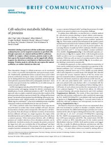
Input The noloco input file is presented in Fig. 2 for the example of the argon dimer. In line 2 one needs to specify the location of the tabulated vdW-DF kernel. The corresponding file kernel.dat can be found in the program source directory. Line 3 contains the information on the flavor of the vdW-DF functional to be used. ‘vdW-DF’ refers to the version by Dion et al. [7], ‘vdW-DF2’ to the latest release by Lee et al. [28], and ‘VV09’ stands for the version by Vydrov and Voorhis [29]. In line 4, the user specifies the size of a supercell which is used for periodic systems to evaluate . The supercell is created as shown in Fig. 3. Here, denote the number of translational images along the three lattice vectors, corresponding to a total number of unit cells
Published as: Comput Phys Commun. 2011 August ; 182(8): 1657–1662.
Nabok et al.
Page 5
(10)
Sponsored Document
Setting equal to corresponds to the case of an isolated molecule, i.e., . In this case, the molecule must be placed at the center of a primitive cell which should be large enough to prevent wave-function overlap with periodic images. Note that noloco does not take into account the symmetry of the cell since typical systems in which vdW interactions play an important role (e.g., molecular crystals or molecule/surfaces interfaces), generally have rather low symmetry. In case of periodic structures, due to the translational symmetry of the electron density, the kernel, and hence the whole integrand, fulfills the condition . Therefore, the region of integration over the variable r runs over one unit cell only, while the integration region for is the supercell. The ultimate size with increasing number of of the supercell is determined by the convergence of translational images , depending on the individual system under investigation. The main parameter required for a Monte-Carlo integration is the requested accuracy of the final value of the integral. This value, which serves as the stopping criterion of the integration, can be chosen either as relative ( , line 5) or absolute accuracy ( , line 6). The integrator tries to find an estimate E (Eq. (7)) for the integral I which fulfills the relation [24].
Sponsored Document
The CUBA library provides the possibility to specify a variety of methods to obtain the integrand estimate: a Korobov [30] or Sobolʼ [31] quasi-random sampling, a Mersenne– Twister [32] pseudo-random sampling, or the cubature rules of Genz and Malik [33]. Here, we use the quasi-random Korobov [30] sequences choosing the number of sampling points in the order of , which is given in line 7. The maximum total number of the integrand evaluations can be specified in line 8. This parameter is only used if the desired convergence has not been reached already. Finally, the name of the file containing the structural data and 3D electron density is specified in line 12. It depends on the code and the underlying band-structure method whether the full density (all-electron codes), the pseudo-density (pseudopotential codes), or the quasi-all-electron density (PAW-based codes) are read in. The flag in line 11 specifies whether the density is given in e/bohr3 or . In line 13, the user can specify a file which contains the density gradients on the same grid as the electron density. In case this data is not available, noloco calculates the density gradients using a three-point formula.
Sponsored Document
4
Applications We illustrate our program with applications to several prototypical vdW-bound systems such as the Ar dimer and graphite, which already have been studied with vdW-DF [7,10,14]. In addition, we provide two more involved examples, the molecular crystal naphthalene [12] as well as thiophene on Cu(110) [16]. We test both reliability and computational efficiency of our implementation. The total energy calculations have been carried out using Quantum ESPRESSO [34]. The information regarding computational time refers to a desktop computer with an Opteron processor, 2.4 GHz and 2 GB RAM. The computational procedure of vdW-DF is a post-scf scheme [7]. In the first step, the crystal or molecular electron density is calculated using the GGA functional according to Perdew, Burke and Ernzerhof (PBE) [35]. In the second step, the non-local correlation
Published as: Comput Phys Commun. 2011 August ; 182(8): 1657–1662.
Nabok et al.
Page 6
energy is evaluated using the self-consistent electron density obtained in the previous step. In the final step, the vdW-DF total energy is determined as (11)
Sponsored Document
We use the vdW-DF flavor [7] in all the examples presented here. Other variants [28,29] are, however, also implemented in our package. 4.1
Argon dimer A typical vdW-bound system, in which standard xc functionals are known to fail, is the Ar dimer. Since the Ar atom has a fully occupied 3p shell, the binding in the dimer is purely due to dispersion forces. Self-consistent calculations were performed by putting two Ar atoms in a cubic supercell of 30 bohr and using a plane-wave energy cutoff of 60 Ry. We first consider the convergence of by choosing different values for the parameter which governs the absolute accuracy of the Monte-Carlo integration (line 6 of the input file). The results are presented in Fig. 4 and Table 1 which also contains the CPU time and the needed to achieve the corresponding accuracy. For comparison, numbers of evaluation the total number of evaluations which would be required by a quadrature rule, , is of
Sponsored Document
order , where , , and are the numbers of grid points along the unit cell vectors where the electron density is represented. As we use 150 points in each direction in this example, is of the order 1013 which corresponds to at least three orders of magnitude higher computing time compared to our approach. Fig. 4 shows the non-local interaction energy for the Ar dimer as a function of the . It turns out that a value of is interatomic distance for different parameters sufficient to obtain converged results. These are in agreement with the corresponding curves from literature [7,36]. 4.2
Graphite Another prototypical vdW system is graphite, for which the interaction between adjacent graphene sheets is of vdW type.
Sponsored Document
For the self-consistent calculations, an energy cutoff of 35 Ry and an k-mesh are used. The in-plane lattice parameter is fixed to the experimental value of , while the inter-plane distance is varied. As mentioned in Section 3, for periodic systems one needs to check the long-range behavior of . The results of such a test is presented in Table 2, where, for simplicity, we only change the lateral supercell size. Note that there are two layers in the unit cell, such that the non-local interaction of the carbon atoms in one plane with those of the other plane is probed. Fortunately, there is almost no dependence of the values larger than (1 1 0). This CPU time on the number of translational images for demonstrates the efficiency of the chosen integration scheme when dealing with periodic systems. The binding energy of the graphene sheets in a graphite crystal as a function of the interlayer distance is presented in Fig. 5.
is calculated using the integration parameters
and . The curves obtained are fully consistent with those previously reported [14]. For comparison, results for some widely used approximate xc functionals are shown also.
Published as: Comput Phys Commun. 2011 August ; 182(8): 1657–1662.
Nabok et al.
4.3
Page 7
Crystalline naphthalene
Sponsored Document
Naphthalene is the simplest representative of the oligoacene family. Its crystal structure is visualized in the center of Fig. 6. The dependence of the non-local energy on the parameter is displayed in the left panel together with the corresponding CPU time for the molecular crystal as well as the isolated molecule computed within the same unit cell. are fixed to . One can see that a value of is sufficient to obtain the non-local energy within 1 mHa. The calculation at this accuracy level only takes around 5 min on a desktop machine. As the computing time, however, increases exponentially with this input parameter, needs to be chosen carefully in case of such complex systems. The right panel is dedicated to the convergence with respect to the number of periodic images. The results for the naphthalene crystal show quick convergence of the non-local energy as a function of the integration volume. It is interesting to note that the characteristic fluctuations of the integral values are of the order of the requested integration accuracy. As in the case of graphite, there is almost no dependence of the computing time on the integration volume. 4.4
Thiophene on Cu(110)
Sponsored Document
As the last example we consider the adsorption of an organic molecule on a metal surface. Thiophene (C4H4S1) on Cu(110) has been studied in detail in Ref. [16] where it turned out that vdW interaction is a substantial contribution to the binding mechanism. We consider a geometry as depicted in the central panel of Fig. 7, with a molecule–metal distance of 2.6 Å. As in the previous case, we test the convergence behavior as a function of the parameter (left panel) and the supercell size (right panel). is required to obtain the nonlocal energy within 0.5 mHa. is found to be sufficient for the same accuracy. Again, the computing time hardly increases with the number of periodic images, but increases exponentially with . Since the electron density is small in the region between the molecule and the surface, a dense grid is required. That would render a geometry relaxation with standard integration techniques for such systems hardly doable.
5
Conclusions
Sponsored Document
We have presented a numerically efficient implementation of the Langreth–Lundqvist vdWDF which is shown to be very useful, in particular, when dealing with periodic systems. The computational efficiency is achieved through the usage of the Monte-Carlo integration technique as implemented in the CUBA library [24]. noloco is freely distributed and can be downloaded from http://amadm.unileoben.ac.at/software.html or http://exciting-code.org. Our code presented here is carefully tested, has different flavors of vdW density functionals included, and can be used on top of any DFT code. So far, it has been used in combination with Quantum Espresso [12,39], Blöchelʼs PAW code [16], VASP [17], exciting [40], Wien2k, and FHI-AIMS [41] being applied to a variety of vdW bound systems, ranging from molecular dimers to surface systems [16,17], molecular crystals and their surface energies [12] as well as for investigating the role of non-local correlations in the coinage metals [41].
References 1. Kohn W. Rev. Mod. Phys.. 1999; 71:1253. 2. Dobson J.F. McLennan K. Rubio A. Wang J. Gould T. Le H.M. Dinte B.P. Aust. J. Chem.. 2001; 54:513. 3. Dobson J.F. Wang J. Dinte B.P. McLennan K. Le H.M. Int. J. Quantum Chem.. 2005; 101:579. 4. Grimme S. J. Comput. Chem.. 2006; 27:1787. [PubMed: 16955487] Published as: Comput Phys Commun. 2011 August ; 182(8): 1657–1662.
Nabok et al.
Page 8
Sponsored Document Sponsored Document Sponsored Document
5. Langreth D.C. Perdew J.P. Solid State Comm.. 1975; 17:1425. 6. Gunnarsson O. Lundqvist B.I. Phys. Rev. B. 1976; 13:4274. 7. Dion M. Rydberg H. Schröder E. Langreth D.C. Lundqvist B.I. Phys. Rev. Lett.. 2004; 92:246401. [PubMed: 15245113] 8. Langreth D.C. Lundqvist B.I. Chakarova-Käck S.D. Cooper V.R. Dion M. Hyldgaard P. Kelkkanen A. Kleis J. Kong L. Li S. Moses P.G. Murray E. Puzder A. Rydberg H. Schröder E. Thonhauser T. J. Phys.: Condens. Matter. 2009; 21:084203. 9. Puzder A. Dion M. Langreth D.C. J. Chem. Phys.. 2006; 124:164105. [PubMed: 16674127] 10. Thonhauser T. Puzder A. Langreth D.C. J. Chem. Phys.. 2006; 124:164106. [PubMed: 16674128] 11. Kleis J. Lundqvist B.I. Langreth D.C. Schröder E. Phys. Rev. B. 2007; 76:100201(R). 12. Nabok D. Puschnig P. Ambrosch-Draxl C. Phys. Rev. B. 2008; 77:245316. 13. Ambrosch-Draxl C. Nabok D. Puschnig P. Meisenbichler C. New J. Phys.. 2009; 11:125010. 14. Chakarova-Käck S.D. Schröder E. Lundqvist B.I. Langreth D.C. Phys. Rev. Lett.. 2006; 96:146107. [PubMed: 16712103] 15. Chakarova-Käck S.D. Borck O. Schröder E. Lundqvist B.I. Phys. Rev. B. 2006; 74:155402. 16. Sony P. Puschnig P. Nabok D. Ambrosch-Draxl C. Phys. Rev. Lett.. 2007; 99:176401. [PubMed: 17995351] 17. Romaner L. Nabok D. Puschnig P. Zojer E. Ambrosch-Draxl C. New J. Phys.. 2009; 11:053010. 18. Gulans A. Puska M.J. Nieminen R.M. Phys. Rev. B. 2009; 79:201105(R). 19. Roman-Perez G. Soler J.M. Phys. Rev. Lett.. 2009; 103:096102. [PubMed: 19792809] 20. Lazic P. Atodiresei N. Alaei M. Caciuc V. Blügel S. Brako R. Comput. Phys. Comm.. 2010; 181:371–379. 21. Davis, P.; Rabinowitz, P. Academic Press; New York: 1975. Methods of Numerical Integration. 22. Press, W.H.; Flannery, B.P.; Teukolsky, S.A.; Vetterling, W.T. Numerical Recipies in Fortran. Vol. vol. 77. Cambridge Univ. Press; 2005. 23. Weinzierl, S. hep-ph/0006269hep-ph/0006269 24. Hahn T. Comput. Phys. Comm.. 2005; 168:78.http://www.feynarts.de/cuba 25. Kokalj A. Comput. Mater. Sci.. 2003; 28:155. Code available from. http://www.xcrysden.org 26. Dion M. Rydberg H. Schröder E. Langreth D.C. Lundqvist B.I. Phys. Rev. Lett.. 2005; 95:109902(E). 27. Gordon W. SIAM J. Numer. Anal.. 1971; 8:158. 28. Lee K. Murray E.D. Kong L. Lundqvist B.I. Langreth D.C. Phys. Rev. B. 2010; 82:081101. 29. Vydrov O.A. Voorhis T.V. Phys. Rev. Lett.. 2009; 103:063004. [PubMed: 19792562] 30. Korobov, N.M. Fizmatgiz; Moscow: 1963. Number-Theoretic Methods of Approximate Analysis. p. 85 (in Russian) 31. Bratley P. Fox B.L. ACM Trans. Math. Software. 1988; 14:88.Sobolʼ I.M. Zh. Vych. Mat. Mat. Fiz.. U.S.S.R. Comput. Math. Math. Phys.. 1967; 1967; 77:784. 86–112. (in Russian). (in English). 32. Matsumoto M. Nishimura T. ACM Trans. Modeling Comp. Simulation. 1998; 8:3. 33. Genz A. Malik A. SIAM J. Numer. Anal.. 1983; 20:580. 34. Giannozzi P. Baroni S. Bonini N. Calandra M. Car R. Cavazzoni C. Ceresoli D. Chiarotti G.L. Cococcioni M. Dabo I. Corso A.D. de Gironcoli S. Fabris S. Fratesi G. Gebauer R. Gerstmann U. Gougoussis C. Kokalj A. Lazzeri M. Martin-Samos L. Marzari N. Mauri F. Mazzarello R. Paolini S. Pasquarello A. Paulatto L. Sbraccia C. Scandolo S. Sclauzero G. Seitsonen A.P. Smogunov A. Umari P. Wentzcovitch R.M. J. Phys.: Condens. Matter. 2009; 21:395502. 35. Perdew J.P. Burke K. Ernzerhof M. Phys. Rev. Lett.. 1996; 77:3865. [PubMed: 10062328] 36. Thonhauser T. Cooper V.R. Li S. Puzder A. Hyldgaard P. Langreth D.C. Phys. Rev. B. 2007; 76:125112. 37. Benedict L.X. Chopra N.G. Cohen M.L. Zettl A. Louie S.G. Crespi V.H. Chem. Phys. Lett.. 1998; 286:490–496. 38. Zacharia R. Ulbricht H. Hertel T. Phys. Rev. B. 2004; 69:155406. 39. Rudenko A.N. Keil F. Katsnelson M.I. Lichtenstein A.I. Phys. Rev. B. 2010; 82:035427.
Published as: Comput Phys Commun. 2011 August ; 182(8): 1657–1662.
Nabok et al.
Page 9
40. Ambrosch-Draxl, C.; Sagmeister, S.; Meisenbichler, C.; Spitaler, J. http://exciting-code.org2009. http://exciting-code.org 41. L. Romaner, X. Ren, C. Ambrosch-Draxl, M. Scheffler, Phys. Rev. Lett. (2011), submitted for publication.
Sponsored Document
Acknowledgments This work was supported by the Austrian Science Fund, project S9714. We thank Lorenz Romaner for careful tests and the implementation of the VV09 functional.
Sponsored Document Sponsored Document Published as: Comput Phys Commun. 2011 August ; 182(8): 1657–1662.
Nabok et al.
Page 10
Sponsored Document
Fig. 1.
The vdW-DF non-local correlation kernel ϕ (multiplied by various values of δ.
Sponsored Document Sponsored Document Published as: Comput Phys Commun. 2011 August ; 182(8): 1657–1662.
) as a function of D for
Nabok et al.
Page 11
Sponsored Document
Fig. 2.
Input file as used for the calculation of the non-local energy contribution for the argon dimer, Fig. 4.
Sponsored Document Sponsored Document Published as: Comput Phys Commun. 2011 August ; 182(8): 1657–1662.
Nabok et al.
Page 12
Sponsored Document
Fig. 3.
Construction of a supercell to evaluate the non-local energy, , for a periodic crystal according to Eq. (1). denote the numbers of translational images along the three lattice vectors. While the variable r is considered in the unit cell (gray area), needs to be taken into account in the whole supercell.
Sponsored Document Sponsored Document Published as: Comput Phys Commun. 2011 August ; 182(8): 1657–1662.
Nabok et al.
Page 13
Sponsored Document
Fig. 4.
Binding energy of the Ar dimer as a function of the interatomic distance, as obtained with the vdW-DF, for different parameters, , governing the accuracy of the Monte-Carlo integration.
Sponsored Document Sponsored Document Published as: Comput Phys Commun. 2011 August ; 182(8): 1657–1662.
Nabok et al.
Page 14
Sponsored Document
Fig. 5.
Binding energy of graphene sheets in graphite as a function of the inter-layer separation. For comparison, we also include results for different xc potentials and experimental data (Exp. 1 [37], Exp. 2 [38]).
Sponsored Document Sponsored Document Published as: Comput Phys Commun. 2011 August ; 182(8): 1657–1662.
Nabok et al.
Page 15
Sponsored Document Fig. 6.
Sponsored Document
Convergence tests for naphthalene. The crystal structure (center) is depicted together with the non-local energy and CPU time as a function of the parameter (left) and the supercell size (right). In the left panel, we used . Results are shown for the crystal as well as for the isolated molecule. In the right panel, data are depicted for and .
Sponsored Document Published as: Comput Phys Commun. 2011 August ; 182(8): 1657–1662.
Nabok et al.
Page 16
Sponsored Document Fig. 7.
Sponsored Document
Convergence tests for thiophene on Cu(110). The adsorption geometry (center) is depicted together with the non-local energy and CPU time as a function of the parameter (left) and the supercell size (right). In the left panel, the integration volume is confined to one unit . cell. In the right panel, the data correspond to
Sponsored Document Published as: Comput Phys Commun. 2011 August ; 182(8): 1657–1662.
Nabok et al.
Page 17
Table 1
Sponsored Document
Non-local correlation energy of the Ar dimer for different parameters which govern the accuracy of the , are Monte-Carlo integration. The corresponding CPU times and numbers of integrand evaluations, included. [Ha]
CPU time [Ha]
10−4
0.18098870
1 min 48 s
0.8⋅108
10−5
0.18097679
8 min 41 s
0.4⋅109
10−6
0.18097998
84 min 55 s
0.2⋅1010
Sponsored Document Sponsored Document Published as: Comput Phys Commun. 2011 August ; 182(8): 1657–1662.
Nabok et al.
Page 18
Table 2
Sponsored Document
Convergence of the non-local correlation energy (in Hartree) of graphite with respect to the number of translational images together with the corresponding CPU time. The parameter has been chosen as CPU time [Ha] (0 0 0)
0.19687
1 min 31 s
(1 1 0)
0.12717
2 min 48 s
(2 2 0)
0.12332
2 min 56 s
(3 3 0)
0.12284
3 min 07 s
(4 4 0)
0.12268
2 min 53 s
(5 5 0)
0.12261
3 min 28 s
Sponsored Document Sponsored Document Published as: Comput Phys Commun. 2011 August ; 182(8): 1657–1662.
.