Computing abstractions of nonlinear systems - arXiv

Gunther Reißig

Computing abstractions of nonlinear systems

1

Computing abstractions of nonlinear systems Gunther Reißig∗

arXiv:0910.2187v3 [math.OC] 15 Feb 2011

Abstract Sufficiently accurate finite state models, also called symbolic models or discrete abstractions, allow one to apply fully automated methods, originally developed for purely discrete systems, to formally reason about continuous and hybrid systems, and to design finite state controllers that provably enforce predefined specifications. We present a novel algorithm to compute such finite state models for nonlinear discrete-time and sampled systems which depends on quantizing the state space using polyhedral cells, embedding these cells into suitable supersets whose attainable sets are convex, and over-approximating attainable sets by intersections of supporting half-spaces. We prove a novel recursive description of these half-spaces and propose an iterative procedure to compute them efficiently. We also provide new sufficient conditions for the convexity of attainable sets which imply the existence of the aforementioned embeddings of quantizer cells. Our method yields highly accurate abstractions and applies to nonlinear systems under mild assumptions, which reduce to sufficient smoothness in the case of sampled systems. Its practicability in the design of discrete controllers for nonlinear continuous plants under state and control constraints is demonstrated by an example. Index Terms Discrete abstraction, symbolic model, nonlinear system, symbolic control, motion planning, formal verification, polyhedral over-approximation, attainability, attainable set; MSC: Primary, 93C10; Secondary, 93C55, 93C57, 93C15, 93B03

I. Introduction In recent years, there has been a growing interest in using finite state models for the analysis and synthesis of continuous and hybrid systems [1]–[9]. This interest has been stimulated by safety critical applications [10], inherent limits of continuous feedback control [11, Sections 5.8-5.10], increasingly complex control objectives [12], and the necessity to cope with the effects of coarse quantization [13]. A sufficiently accurate finite state model, also called a symbolic model or discrete abstraction, would allow one to apply fully automated methods, originally developed for purely discrete systems [14]–[16], to formally reason about the original system, and to design finite state controllers that provably enforce predefined specifications [2]–[9]. Obtaining such abstractions constitutes a challenging problem, which has only been satisfactorily solved for special cases. Under the name symbolic dynamics, finite state models of continuous systems had already been a well-established mathematical tool [17] when the concept appeared in the engineering literature [18], [19]. Much of the subsequent research has been devoted to systems whose continuous-valued dynamics is linear. Methods for nonlinear systems have been systematically studied since around 1980; see [1], [4]–[9]. In the earliest ∗

Universit¨ at Kassel, Fachbereich 16 - Elektrotechnik/Informatik, Regelungs- und Systemtheorie, Wilhelmsh¨ oher Allee 73, D-34121 Kassel, Germany, http://www.reiszig.de/gunther/ This work has been accepted for publication in the IEEE Trans. Automatic Control. Copyright may be transferred without notice, after which this version may no longer be accessible. Please refer to author’s homepage and to IEEE Xplore for the definite publication. You may also find a BibTEX entry at the former website.

Gunther Reißig


2

such approach [20], attainable sets are approximated by means of trajectories emanating from a finite set of initial points, hence the name sampling method [20]. This method has been successfully applied to a variety of problems [1], [4]–[8], [21]–[23], including symbolic control of sampled systems [23], [24]. An extension allows for rigorous overapproximation of attainable sets [25], and thus, for the computation of abstractions. Over the years, a large number of alternatives to the sampling method have been proposed, which represent a variety of compromises between approximation accuracy, practicability, rigor, and computational complexity [23], [26]–[42]. In the present paper, we aim at computing abstractions for nonlinear discrete-time systems of the form xk+1 = G(xk , uk ), (1) where the state x takes values in a subset of Rn , and u is an input signal which is assumed to take its values in some finite set U. If (1) arises from a continuous-time system x˙ = F (x, v)

(2)

under sampling, its right hand side G may not be explicitly given. Our results will still apply as we will formulate hypotheses to be verified and computations to be performed directly in terms of the right hand side F of (2). The approach we follow involves quantizing the state space of (1) with the help of a finite covering C of Rn whose elements we call cells [1]–[9]. The system (1) is supplemented with a quantizer Q which assigns to any state x of (1) the collection of those cells in C that contain x, Q(x) = {∆ ∈ C | x ∈ ∆}. That is, a pair (u, ∆) of an input signal u0 , u1 , . . . and an output signal ∆0 , ∆1 , . . . could possibly be generated by the quantized system composed of (1) and the non-deterministic output relation ∆k ∈ Q(xk )

(3)

iff there exists a sequence x0 , x1 , . . . such that (1) and (3) hold for all non-negative integers k 1 . The collection of such pairs (u, ∆) is called the behavior of the quantized system (1),(3) [43]. The input alphabet U and the output alphabet C of the quantized system (1),(3) are both finite. Control problems for (1),(3) can still be challenging to solve, especially if the system (1) is nonlinear and the specification involves constraints or is otherwise complex. In contrast, controllers (or supervisors) for finite automata are generally straightforward to design [14], [16], which raises the question of whether controllers for the quantized system (1),(3) can be obtained by solving auxiliary control problems for automata that approximate the behavior of (1),(3). As it turns out, this strategy is feasible if the approximation is both conservative and sufficiently precise, e.g. [3], [44]–[46]. That is, the automaton must be capable of generating any signal in the behavior of (1),(3), and the set of spurious signals should be small. In other words, the said strategy requires a discrete abstraction, by which we mean a superset of the behavior of (1),(3) that can be realized by a finite automaton, and this abstraction should be as accurate as possible. One way to prescribe the accuracy of an abstraction is to restrict the extent by which its signals are allowed to violate the dynamics of (1),(3). While, by definition, signals in the behavior of the quantized system (1),(3) are consistent with the dynamics of (1),(3) at all times, a common class of abstractions require consistency only on finite 1 The symbols u, x and ∆ are used to denote elements of U , Rn and C, respectively, as well as signals taking their values in these sets.

Gunther Reißig


x0

∆t+2 ∆t+1 G(·, ut ) xt xt+1 G(·, ut+1 ) xt+2 ∆t (a)

∆t+N xt+N

∆0 −2

G(·, u0 )

3

1

−1 ∆ x1 1 −1

1

2

G(·, u1 )

∆2

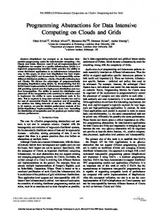
(b) Figure 1. (a) Illustration of consistency with the dynamics of the quantized system (1),(3) on finite time intervals. (b) Quantizer cells may serve as states of automata realizations of abstractions of memory span 1, where transitions are defined by condition (4).

time intervals [44], [45]. Such an abstraction contains any pair (u, ∆) that fulfills the following condition, in which the memory span N ≥ 1 determines the accuracy [43]: For any non-negative integer t there are states xt , . . . , xt+N such that (1) and (3) hold for all k ∈ {t, t + 1, . . . , t + N − 1} and k ∈ {t, t + 1, . . . , t + N}, respectively. See Fig. 1(a). In the case that N = 1, consistency of (u, ∆) is equivalent to the existence of a sequence x0 , x1 , . . . for which xk ∈ ∆k and G(xk , uk ) ∈ ∆k+1 (4) hold for all k. Hence, the cells in the covering C may serve as states of an automaton realization of the abstraction, where the occurrence of an input symbol uk ∈ U enables a transition from ∆k ∈ C to ∆k+1 ∈ C iff there is a state xk of (1) such that (4) holds. Obviously, that automaton will be capable of generating any pair of signals u and ∆ in the behavior of (1),(3). The fact that it will generally also generate spurious signals is illustrated in Fig. 1(b). If (1) requires the sign of the second component of the state to be constant, then the sequence ∆0 , ∆1 , ∆2 , . . . of cells generated by the automaton is not consistent with the dynamics of (1),(3). In contrast, consistency of (u, ∆) for N > 1 requires, amongst other conditions, that (4) holds with x1 = G(x0 , u0), which rules out the spurious signal ∆0 , ∆1 , ∆2 , . . . of Fig. 1(b). Indeed, increasing the memory span N generally results in more accurate abstractions. In this paper we shall present a novel algorithm to compute abstractions of finite but otherwise arbitrary memory span that builds on a well-known reformulation of consistency on finite time intervals in terms of attainable sets [44], [45], on a new method to compute polyhedral over-approximations of the latter, and on new results that guarantee the convexity of attainable sets of (1) and (2). In our approach, polyhedral quantizer cells are embedded into suitable supersets whose attainable sets under the dynamics of (1) are convex for the duration of N time steps, where N is the memory span of the abstraction that is being computed. That convexity requirement permits us to over-approximate attainable sets by intersections of supporting half-spaces, and the latter are obtained from systems of linear equations derived from (1). The number of half-spaces needed can be quite large, especially if the memory span exceeds 1. We present a novel recursive description of these half-spaces and propose an iterative procedure to compute them efficiently. The existence of the aforementioned embeddings of quantizer cells is, in fact, the essential requirement for our method to apply. The results in this paper not only allow verification of that requirement when a particular quantizer is given, but they also show how to meet it using sufficiently small but otherwise arbitrary polyhedral cells. We use

Gunther Reißig


4

strongly convex supersets of quantizer cells, and the error by which we over-approximate attainable sets depends quadratically on the size of the cells. Application of our earlier results [47], [48] on ellipsoidal supersets would have led to linear error bounds. Thus, the accuracy of the computed abstractions is improved if a particular quantizer is given. Alternatively, fewer and larger cells may be used, which reduces the computational effort to compute abstractions and also reduces the complexity of controllers designed on the basis of the latter. These results are obtained under mild assumptions on the right hand side G of (1), which reduce to sufficient smoothness in the case of sampled systems. The remaining of this paper is organized as follows. The next section introduces basic notation and terminology. In Section III we present our algorithm for the computation of abstractions, prove its correctness, and analyze its computational complexity. Section IV is devoted to our results on the convexity of attainable sets. In Section V, practicability of our approach in the design of discrete controllers for nonlinear continuous plants under state and control constraints is demonstrated by an example. We also present computational results on how the computational effort of our approach grows with the problem size. II. Preliminaries A. Basic notation R and Z denote the sets of real numbers and integers, respectively, R+ and Z+ , their subsets of non-negative elements, and N = Z+ \ {0}. [a, b], ]a, b[, [a, b[, and ]a, b] denote closed, open and half-open, respectively, intervals with end points a and b, e.g. [0, ∞[ = R+ . [a; b], ]a; b[, [a; b[, and ]a; b] stand for discrete intervals, e.g. [a; b] = [a, b] ∩ Z. For any sets A and B, f : A → B denotes a map of A into B, and B A is the set of all such maps. Operations involving subsets of Rn are defined pointwise [49, Appendix A], e.g. ∆ + ∆′ := {ω + ω ′ | ω ∈ ∆, ω ′ ∈ ∆′ } and ϕ([0, t] , ∆) := {ϕ(τ, ω) | τ ∈ [0, t] , ω ∈ ∆} if ∆, ∆′ ⊆ Rn , ϕ : R × Rn → Rn , and t ∈ R. C k denotes the class of k times continuously differentiable maps, and C k,1, the class of maps in C k with (locally) Lipschitz-continuous kth derivative. B. Behaviors Given an arbitrary set W called signal alphabet, any subset B ⊆ W Z+ is a behavior on W [43]–[46], [50]. Hence, elements of B are infinite sequences w : Z+ → W , which we call signals. We denote the value of the signal w at time k by wk . The backward τ -shift σ τ is defined by (σ τ w)k = wτ +k . The restriction of B to I ⊆ Z+ , B|I , is defined by B|I := {w|I | w ∈ B}. B is time-invariant if σ1 B ⊆ B. B is N-complete, or equivalently, B has memory span N, if N ∈ Z+ and B = w ∈ W Z+ ∀τ ∈Z+ (σ τ w)|[0;N ] ∈ B|[0;N ] . A superset B ′ of a behavior B ⊆ W Z+ is called an abstraction of B, and B ′ is additionally called discrete if it can be realized by a finite automaton. C. Discrete-time systems In (1) with right hand side G : X × U → X, u : Z+ → U represents an input signal and x : Z+ → X, a state signal. A trajectory of (1) is a sequence (x, u) : Z+ → X × U for which (1) holds for all k ∈ Z+ . The collection of such trajectories, which is a subset of (X × U)Z+ , is called the behavior of (1). The general solution ψ : Z+ × X × U Z+ → X of (1) is the map defined by the requirement that (ψ(·, x0 , u), u) is a trajectory of (1) and

Gunther Reißig


5

ψ(0, x0 , u) = x0 . Of course, it is not necessary to specify u on the whole time axis, so we may write ψ(k, x0 , u0, . . . , uk′−1 ) := ψ(k, x0 , u|[0,k′ [ ) := ψ(k, x0 , u) whenever k ′ ≥ k. We will often assume the following. (H1 ) X ⊆ Rn is open and G : X × U → X is such that for all u ∈ U, the map G(·, u) is a C 1 -diffeomorphism onto an open subset of X. We will say (H1 ) is fulfilled with smoothness C K if (H1 ) holds with G(·, u) of class C K rather than merely C 1 . III. Computation of abstractions In the present section, we shall develop an efficient algorithm for computing abstractions of (1) that can be represented by finite automata. Intuitively, our approach is that of successively expanding the behavior of (1) and may be seen to comprise four approximation steps: State space quantization, approximation by the smallest discrete abstraction, approximation by a collection of convex programs, approximation by a collection of linear programs. The purpose of state space quantization is to conservatively approximate (1) using a finite signal alphabet, which is an important prerequisite for a finite automaton approximation. Unfortunately, 1-completeness of the behavior of (1) is usually lost, and in general the behavior of the quantized system is not N-complete for any N. In order to reintroduce N-completeness, which is sufficient for a finite automaton representation to exist, we approximate the quantized system again, this time by the smallest discrete abstraction of memory span N. A problem with the latter abstraction is that it may only be computed exactly for special cases of both systems (1) and state space quantizations. Two more approximation steps yield further abstractions, which are both N-complete and characterized in terms of computationally tractable problems. Specifically, we first replace each quantizer cell by a suitable superset whose attainable sets are known to be convex, and then determine tight polyhedral over-approximations, i.e., collections of supporting half-spaces, of the latter. This yields abstractions characterized in terms of linear programs. As it turns out, each half-space can be obtained as a solution of a system of linear equations derived from (1) and of differential equations derived from (2), respectively. A. State space quantization Quantization of the state space of (1) is realized by supplementing (1) with a quantizer; see Section I. The system C of quantizer cells is chosen as follows. We first define a region K of the state space X of (1) whose local dynamics is deemed an essential part of the behavior of (1), then choose a finite covering C ′ of K, and finally supplement C ′ by additional cells in order to obtain a covering C of Rn . Intuitively, K is the intended operating range of the quantizer, whereas cells in C \ C ′ represent overflow symbols. Of course, what is considered essential local dynamics depends on the purpose of our analysis of (1), and our choice of C ′ will also be influenced by other particularities of the problem at hand; hence a general rule for the choice of the quantizer cannot be given. However, the following hypothesis should be fulfilled in order to ensure the correctness of the algorithm for the computation of abstractions we are going to present.

Gunther Reißig


6

(H2 ) The input alphabet U is finite, and C is a finite covering of Rn whose elements are b in nonempty convex polyhedra. For each cell ∆ ∈ C ′ ⊆ C there is a superset, denoted ∆ b b the sequel, for which ∆ ⊆ X and attainable sets ψ(k, ∆, u) are convex for all k ∈ [1; N] and all u : [0; k[ → U, where ψ denotes the general solution of (1), and N, the memory span of the abstraction we seek to obtain. In the present section, the above condition plays the role of an assumption. The nontrivial question of how to verify it is postponed to Section IV. B. Smallest discrete abstractions Let B ⊆ (U ×C)Z+ denote the behavior of the quantized system (1),(3), and let N ∈ Z+ be given. The N-complete hull BN of B is the intersection of all N-complete behaviors B ′ ⊆ (U × C)Z+ that contain B as a subset. Under the name strongest N-complete approximations, N-complete hulls have been introduced and investigated by Moor and his collaborators, e.g. [44], [45]. It has been shown that B ⊆ BN +1 ⊆ BN and that Ncomplete hulls are indeed N-complete.Thus, the map that assigns to B its N-complete hull BN is a closure operator [51], and BN is the smallest discrete abstraction of memory span N of B. Moreover, BN admits the following characterization [44], [45]. III.1 Proposition. Let C be a covering of Rn , N ∈ Z+ , u : [0; N] → U, ∆ : [0; N] → C, ψ the general solution of (1), B the behavior of the quantized system (1),(3), and BN the N-complete hull of B. Then BN = w : Z+ → W ∀τ ∈Z+ (σ τ w)|[0;N ] ∈ B|[0;N ] . Moreover, the sets M0 , . . . , MN defined by Mk = ψ(k, x0 , u) x0 ∈ X, ∀τ ∈[0;k] ψ(τ, x0 , u) ∈ ∆τ

(5)

satisfy Mk = ∆k ∩ G(Mk−1 , uk−1 ) for all k ∈ [1; N], and for all k ∈ [0; N] we have (u, ∆) ∈ B|[0;k] iff Mk = 6 ∅. In view of Proposition III.1, computing an exact representation of the k-complete hull Bk of the behavior of (1),(3) would require verifying Mk (u, ∆) 6= ∅

(6)

for all choices of sequences u and ∆, where Mk (u, ∆) is defined by the right hand side of (5). To verify (6), in turn, one must check whether there is some initial point x0 ∈ ∆0 such that the trajectory generated by x0 and u visits ∆1 , . . . , ∆k at times 1, . . . , k; see also Fig. 1(a). (In fact, Mk (u, ∆) consists of the values at time k of the trajectories that satisfy the latter condition.) To perform that test is, in general, an extremely difficult problem which may only be exactly solved in rather special situations. One therefore aims at efficiently computing discrete abstractions that conservatively approximate the smallest one, Bk , and resort to a test ck (u, ∆) 6= ∅ M

(7)

ck (u, ∆) of Mk (u, ∆), e.g. [28]. On the one hand, the set for some outer approximation M c(u, ∆) should have a simple structure in order to allow for efficiently testing condition M (7). On the other hand, that set should approximate M(u, ∆) as accurately as possible, since Bk already is an over-approximation of the actual behavior of the quantized system

Gunther Reißig


7

c(u, ∆) \ M(u, ∆) will inevitably lead to additional spurious (1),(3) and the difference M signals. The following novel characterization of Bk , which is not valid in the more general setting ck (u, ∆). of [44], [45], will be crucial in our determination of suitable candidates for M

III.2 Proposition. Let C, N, u, ∆, ψ and Mk be as in Proposition III.1 and assume in addition that G(·, u) is injective for all u ∈ U. Then Mk =

k \

τ =0

for all k ∈ [0; N].

ψ(τ, X ∩ ∆k−τ , u|[k−τ ;k[ )

(8)

Proof. (8) obviously holds for k ∈ {0, 1}, so assume (8) holds for some k ∈ [1; N[. Then, using Proposition III.1, we obtain ! k \ Mk+1 = ∆k+1 ∩ G(Mk , uk ) = ∆k+1 ∩ G ψ(τ, X ∩ ∆k−τ , u|[k−τ ;k[), uk . τ =0

Injectivity of G(·, uk ) implies G(A ∩ B, uk ) = G(A, uk ) ∩ G(B, uk ) for any sets A and B. This together with G(ψ(τ, ·, u|[k−τ ;k[ ), uk ) = ψ(τ + 1, ·, u|[k−τ ;k]) gives Mk+1 = ∆k+1 ∩ = ∆k+1 ∩

k \

τ =0 k+1 \

τ =1

ψ(τ + 1, X ∩ ∆k−τ , u|[k−τ ;k+1[) ψ(τ, X ∩ ∆k+1−τ , u|[k+1−τ ;k+1[).

C. Polyhedral over-approximations of attainable sets endow the space Rn with the standard Euclidean product h·|·i, i.e., hx|yi = PWe n n i=1 xi yi for any x, y ∈ R . The derivative and the inverse of a map f is denoted ′ −1 by f and f , respectively, and f ∗ is the transpose of f if f : Rn → Rm is linear. III.3 Definition. For any C 1 -diffeomorphism Φ : V → W between open sets V, W ⊆ Rn , the complementary extension Φ♦ : V × Rn → W × Rn of Φ is defined by ∗ Φ♦ (p, v) = Φ(p), Φ′ (p)−1 v . We further define

for all p, v ∈ Rn and set

P (p, v) = {x ∈ Rn | hv|x − pi ≤ 0}

(9)

\

(10)

P (Σ) =

P (p, v)

(p,v)∈Σ n

n

for Σ ⊆ R × R . In words, (10) is the intersection of the half-spaces (9) represented by pairs (p, v) ∈ Σ. III.4 Definition. A vector v ∈ Rn is normal to Ω ⊆ Rn at a boundary point p of Ω if hv|x − pi ≤ 0 for all x ∈ Ω. We call Σ an outer convex approximation of Ω if Ω ⊆ P (Σ), and a supporting convex approximation of Ω, if p ∈ Ω and v is normal to Ω at p, for all (p, v) ∈ Σ. A finite outer (supporting, resp.) convex approximation is polyhedral.

Gunther Reißig


8

ck (u, ∆) for the test (7). If Let us now return to the problem of suitable candidates M ck (u, ∆) to be hypothesis (H2 ) holds and ∆0 , . . . , ∆N ∈ C ′ , we could define M bk ∩ ∆

k \

τ =1

b k−τ , u|[k−τ ;k[ ), ψ(τ, ∆

(11)

b N and all the sets ψ(τ, ∆ b N −τ , u|[N −τ,N [ ) are convex by (H2 ), the test (7) would and since ∆ be a convex program. The strategy we actually pursue is to take some suitable outer ck (u, ∆). Then the convex program (7) becomes polyhedral approximation of (11) for M ck (u, ∆) enjoy a recursive description. linear, and the sets M

III.5 Proposition. Assume (H2 ) for some N ∈ Z+ , as well as (H1 ), and let ∆ : [0; N] → C ′ , u : [0; N[ → U and Σ, S : [0; N] → P(Rn × Rn ), where P(·) denotes the power set. b k for all k ∈ [0; N], Assume further that Σk is a supporting convex approximation of ∆ and S0 = Σ0 ,

(12)

♦

Sk = Σk ∪ G(·, uk−1) (Sk−1) for k ∈ [1; N].

(13)

Then, for all k ∈ [1; N], G(·, uk−1)♦ (Sk−1 ) is an outer convex approximation of T k b τ =1 ψ(τ, ∆k−τ , u|[k−τ ;k[ ), and in particular, Sk is one of (11). ck (u, ∆) The above result will enable us to iteratively and efficiently compute the sets M defined earlier. For given u and ∆, such sets correspond to P (Sk ), i.e., to the intersection of the half-spaces represented by pairs (p, v) ∈ Sk of points p and normals v. In view ck (u, ∆) is the intersection, of this implicit representation of polyhedra, (13) says that M ♦ and not the union, of polyhedra P (Σk ) and P (G(·, uk−1) (Sk−1 )). Moreover, in contrast ck (u, ∆) is not the intersection of attainable sets of quantizer cells to Mk (u, ∆), the set M under the dynamics of (1), which is why Propositions III.1 and III.2 cannot be applied to obtain the recursive description in Proposition III.5. To prove Proposition III.5 we need the following auxiliary result.

III.6 Lemma. Assume Φ : V → W is a C 1 -diffeomorphism between open sets V, W ⊆ Rn such that both Ω ⊆ V and Φ(Ω) are convex, and let p ∈ Ω. ∗ Then v ∈ Rn is normal to Ω at p iff (Φ′ (p)−1 ) v is normal to Φ(Ω) at Φ(p). In particular, Σ ⊆ Rn × Rn is a supporting convex approximation of Ω iff Φ♦ (Σ) is one of Φ(Ω). ∗

Proof. Let v be normal to Ω at p and define w = (Φ′ (p)−1 ) v and q = Φ(p) as well as γ : [0, 1] → Rn : t 7→ Φ−1 (q + t(y − q)) for some y ∈ Φ(Ω). The map γ is well-defined, differentiable and takes its values in Ω since q, y ∈ Φ(Ω) and Φ(Ω) is convex. This implies the map α defined by α(t) = hv|γ(t) − pi is non-positive as v is normal to Ω at p. ′ Furthermore, α is differentiable with α(0) = 0, hence 0 ≥ α′ (0) = v (Φ−1 ) (q)(y − q) = hw|y − qi. As y is an arbitrary element of Φ(Ω), w is normal to Φ(Ω) at q. ∗ For the converse assume w is normal to Φ(Ω) at q and observe (((Φ−1 )′ (q))−1 ) w = v. The first part of this proof applied to Φ−1 then shows that v is normal to Ω at p. Proof of Proposition III.5. Let v : Z+ → U and observe that ψ(0, p, v) = p and ψ(k + 1, p, v) = G(ψ(k, p, v), vk ) for all k ∈ Z+ and all p ∈ X. Then, by induction, ψ(k, ·, v) is a C 1 -diffeomorphism between X and an open subset of X, which has two implications. First, by (H2 ) and Lemma III.6, ψ(τ, ·, u|[k−τ ;k[ )♦ (Σk−τ ) is a supporting convex

Gunther Reißig


9

G(·, u)♦ b P (G(·, u)♦ (Σ(∆)))

G(·, u)

∆

G(∆, u) b P (Σ(∆))

b ∆

b u) G(∆,

Figure 2. Approximation principle underlying the algorithm in Fig. 3: Let u ∈ U and consider a cell ∆ ∈ C ′ whose image G(∆, u) under the nonlinear map G(·, u) is non-convex. ∆ is conservatively approximated b and ∆ b in turn, by a supporting convex polyhedron P (Σ(∆)). b b is mapped under the by some set ∆, Σ(∆) complementary extension G(·, u)♦ . The result, in contrast to images under G(·, u), again represents a convex b b u) is convex, which guarantees G(∆, u) ⊆ G(∆, b u) ⊆ polyhedron, P (G(·, u)♦ (Σ(∆))). By hypothesis (H2 ), G(∆, b P (G(·, u)♦ (Σ(∆))). The latter set is the one that is actually computed.

b k−τ , u|[k−τ ;k[) for all k ∈ [0; N] and all τ ∈ [0; k]. Second, we have approximation of ψ(τ, ∆ ψ(k + 1, ·, v)♦ = G(·, vk )♦ ◦ ψ(k, ·, v)♦

(14)

for all k ∈ Z+ , where ◦ denotes composition [51], since obviously (Φ ◦ Ψ)♦ = Φ♦ ◦ Ψ♦ for any diffeomorphisms Φ and Ψ whose composition Φ ◦ Ψ is well-defined. We now show G(·, uk−1)♦ (Sk−1 ) =

k [

τ =1

ψ(τ, ·, u|[k−τ ;k[ )♦ (Σk−τ )

(15)

for all k ∈ [1; N], which proves the proposition. Observe first that (12) implies (15) for k = 1, and then assume (15) holds for some k ∈ [1; N[. Then G(·, uk )♦ (Sk ) equals ♦

G(·, uk ) (Σk ) ∪

k [

τ =1

G(·, uk )♦ (ψ(τ, ·, u|[k−τ ;k[)♦ (Σk−τ ))

by (13). The first set in this union is ψ(1, ·, u|[k;k+1[ )♦ (Σk ), and by (14), the union of the S last k sets equals kτ=1 ψ(τ + 1, ·, u|[k−τ ;k+1[ )♦ (Σk−τ ). This implies (15) with k replaced by k + 1. D. Algorithmic solution We now present an algorithm for efficiently computing discrete abstractions for the quantized system (1),(3), which is based on the geometric idea behind Prop. III.5. See also Fig. 2. Since we are now investigating behaviors, which are sets of signals (u, ∆), the analogs of the sets Sk introduced in Proposition III.5 will depend on u and ∆, which is why we denote them by S(u|[τ ;τ +k[ , ∆|[τ ;τ +k] ) in what follows. b be a III.7 Theorem. Let be n ∈ N and N ∈ Z+ , assume (H1 ) and (H2 ) hold, let Σ(∆) S N ′ [0;k[ b for all ∆ ∈ C , and let the map S : supporting polyhedral approximation of ∆, × k=0 U C [0;k] → P(Rn × Rn ) be defined by the output of the algorithm in Fig. 3. Then, for all k ∈ [0; N], the set (u, ∆) ∈ (U × C)Z+ ∀τ ∈Z+ P (S(u|[τ ;τ +k[ , ∆|[τ ;τ +k] )) 6= ∅ , which is denoted Bk , is a k-complete discrete abstraction of the behavior of the quantized system (1),(3).

Gunther Reißig


10

b for each ∆ ∈ C ′ . Input: n, N, U, G, C, C ′ ; Σ(∆) 1: for all ∆ ∈ ( C do b Σ(∆), if ∆ ∈ C ′ , 2: S(∆) := ∅, otherwise 3: end for 4: for k = 0, . . . , N − 1 do 5: for all u : [0; k + 1[ → U, ∆ : [0; k + 1] → C do 6: if S(u|[0;k[ , ∆|[0;k] ) = ∅ then 7: S(u, ∆) := ∅ 8: else if ∆k+1 ∩ P (G(·, uk )♦ (S(u|[0;k[ , ∆|[0;k] ))) = ∅ then 9: S(u, ∆) := Rn × Rn 10: else if ∆k+1 ∈ / C ′ then 11: S(u, ∆) := ∅ 12: else b k+1 ) ∪ G(·, uk )♦ (S(u|[0;k[ , ∆|[0;k] )) 13: S(u, ∆) := Σ(∆ 14: end if 15: end for 16: end for Output: S Figure 3. Algorithm for the computation of outer polyhedral approximations of attainable sets that define a discrete abstraction of quantized system (1),(3).

Proof. First observe the operations to be performed by the algorithm in Fig. 3 are welldefined. In particular, G(·, uk )♦ on lines 8 and 13 of the algorithm shown in Fig. 3 is b k+1 ) on line 13 is as well, by the test well-defined by hypotheses (H1 ) and (H2 ), and Σ(∆ on line 10. Denote the behavior of quantized system (1),(3) by B. In order to show Bk is kcomplete, let u : Z+ → U and ∆ : Z+ → C, and assume that for all τ ∈ Z+ there is some (v, Γ) ∈ Bk such that (σ τ u)|[0;k] = v|[0;k] and (σ τ ∆)|[0;k] = Γ|[0;k] . This implies ∅= 6 P (S(v|[0;k[ , Γ|[0;k] )) = P (S(u|[τ ;τ +k[, ∆|[τ ;τ +k])), thus (u, ∆) ∈ Bk . Given arbitrary K ∈ [0; N[, u : [0; K + 1[ → U and ∆ : [0; K + 1] → C, we now show P (S(u|[0;k[ , ∆|[0;k] )) = ∅ implies Mk = ∅

(16)

for all k ∈ [0; K + 1], where Mk is defined by (8). According to Propositions III.1 and III.2, this implies B ⊆ Bk , and hence, proves the theorem. From the initialization of S on lines 1-3 of the algorithm and hypothesis (H2 ) it follows that P (S(∆0 )) 6= ∅, thus (16) holds for k = 0. Assume now that (16) holds for all k ∈ [0; K], for some K ∈ [0; N[, as well as P (S(u, ∆)) = ∅. In view of lines 6 and 7, this implies S(u|[0;k[ , ∆|[0;k] ) 6= ∅ for all k ∈ [0; K + 1]. We further obtain ∆k+1 ∩ P (G(·, uk )♦ (S(u|[0;k[ , ∆|[0;k] ))) = ∅

(17)

for k = K. Otherwise, S(u, ∆) would have been assigned its value on line 13, i.e., b k+1 ) ∪ G(·, uk )♦ (S(u|[0;k[ , ∆|[0;k] )) S(u|[0;k+1[ , ∆|[0;k+1] ) = Σ(∆

(18)

Gunther Reißig


11

for k = K; thus the left hand side of (17) would be a subset of P (S(u, ∆)) = ∅, which is a contradiction. Now assume (17) also holds for some k ∈ [0; K[. Then S(u|[0;k+1[ , ∆|[0;k+1] ) is assigned its value on line 9, hence P (S(u|[0;k+1[ , ∆|[0;k+1] )) = ∅. From this and (16) we obtain Mk+1 = ∅, and Proposition III.1 yields MK+1 = ∅. Thus, (16) holds for k = K + 1. If, on the other hand, (17) does not hold for any k ∈ [0; K[, then, in view of lines 2, b 0 ), as well as (18) 6, 7, 10 and 11, we obtain ∆τ ∈ C ′ for all τ ∈ [0; K], S(∆0 ) = Σ(∆ for all k ∈ [0; K[. Proposition III.5 then shows that the left hand side of (17) for k = K contains MK+1 as a subset, so (16) holds for k = K + 1, and we are done. III.8 Corollary. Under the hypotheses of Theorem III.7 and for all k ∈ [0; N], the requirement ∃∆ : Z+ →C (u, ∆) ∈ Bk and ∀k∈Z+ xk ∈ ∆k

for sequences (u, x) : Z+ → U × Rn defines an abstraction of the behavior of the discretetime system (1). We remark that the algorithm in Fig. 3 contains just two nontrivial operations which need to be performed repeatedly, namely, the determination of the set G(·, uk )♦ (S(u|[0;k[ , ∆|[0;k] )),

(19)

which appears on lines 8 and 13, and the test for emptiness on line 8. The latter can be efficiently performed using linear programming techniques, since both ∆k+1 and P (G(·, uk )♦ (S(u|[0;k[ , ∆|[0;k] ))) are convex polyhedra. According to Definition III.3, the former operation requires an evaluation of the function G(·, uk ) and the solution of a linear system of equations for each element (p, v) ∈ S(u|[0;k[ , ∆|[0;k] ), p˜ = G(p, uk ),

(20a) ∗

v = D1 G(p, uk ) v˜,

(20b)

in order to obtain an element (˜ p, v˜) of (19), which represents one half-space in the outer convex approximation (19). Here, Di f denotes the partial derivative of f with respect to the ith argument. In order to estimate the computational complexity of the algorithm in Fig. 3, we assume b is approximated by m supporting half-spaces, i.e., for simplicity that each of the sets ∆ ′ b for all ∆ ∈ C , where | · | denotes cardinality. It is then easy to see that for m = |Σ(∆)| any given k ∈ [0; N[, the number of half-spaces needed to define all the sets (19) is at most m|C||U|k+1, and these sets are represented by at most (k + 1)m half-spaces each. To estimate the number of tests for emptiness, we additionally assume that there is a constant λ > 0, independent of |C|, such that the following holds. For any given set of the form (19), the test on line 8 has to be performed for at most λ cells ∆k+1 ∈ C, and the set of these candidate cells can be provided in constant time. This holds, in particular, if the cells in C ′ are congruent compacta arranged in a regular grid. Then, for any given k, the number of tests on line 8 is bounded by λk+1 |C||U|k+1. Note here that the values ∅ and Rn × Rn , which may be assigned on lines 9 and 11, play a role similar to zeros in sparse matrices, and thus, these values do not need to be stored and computations on them do not need to actually be performed [52]. In summary, the algorithm in Fig. 3 requires the solution of O(m|C||U|N ) instances of (20) and of O(λN |C||U|N ) linear feasibility problems in n variables with at most (N +1)m inequalities each, where O(·) is the usual asymptotic notation [53]. The parameters m

Gunther Reißig


12

and |C| depend on the dimension n of the state space of (1), with |C| typically growing exponentially. Therefore, the computational effort has to be expected to grow rapidly with n, a problem that is common to all grid based methods for the computation of abstractions, e.g. [1], [8], [26], [27], [32]. We remark that apart from an increasing computational effort, application of the algorithm shown in Fig. 3 in dimensions exceeding 2 does not pose any particular difficulties. This is obvious for the operations on lines 8 and 13, which we have already discussed, and also holds for the remaining operations. Specifically, for the computation of the b on line 2, several methods are available for supporting polyhedral approximations Σ(∆) b [53]. a large class of sets ∆ Finally, we would like to emphasize again that convexity of certain attainable sets is an important requirement for the correctness of the algorithm in Fig. 3, see hypothesis b = ∆, the (H2 ). While for linear systems that requirement is always met by the choice ∆ results of section IV will show how to meet it in the presence of non-linearities. E. Sampled systems Here we consider the case that (1) arises from a continuous-time system (2) under sampling. More formally, let a continuous-time control system (2) with F : X × V → Rn and a set U of input signals be given, where X ⊆ Rn , V ⊆ Rm , each u ∈ U is a piecewise continuous map u : [0, T ] → V , and T > 0 is the sampling period . A map v : R+ → V is an admissible input signal for (2), generated by u : Z+ → U, if v(t) = uk (t − kT ) for all k ∈ Z+ and all t ∈ [kT, (k + 1)T [. The set of admissible input signals for (2) is denoted V in the sequel. We assume the following. (H3 ) X ⊆ Rn is open, the right hand side F of (2) is continuously differentiable with respect to its first argument and continuous. Furthermore, for any x0 ∈ X and any admissible input signal v ∈ V, the solution of the initial value problem composed of (2) and the initial condition x(0) = x0 is extendable to the entire time axis R+ . Discrete-time system (1) is called the sampled system associated with (2) if its right hand side is given by G(x, u) = ϕ(T, x, u) for all x ∈ X and all u ∈ U, where ϕ is the general solution of (2), i.e., ϕ(t, x0 , v) is the value at time t of the solution of the initial value problem composed of (2) and the initial condition x(0) = x0 . Obviously, the sampled system (1) associated with (2) fulfills (H1 ) if (2) fulfills (H3 ), and ψ(k, x, u) = ϕ(kT, x, v) for all x ∈ X and all k ∈ Z+ , whenever v is an admissible input signal for (2) generated by the sequence u : Z+ → U and ψ is the general solution of (1). Hence, our results for (1), including the algorithm in Fig. 3, can be directly applied to the sampled system (1) associated with (2) if the latter satisfies hypothesis (H3 ). In particular, (20) can be efficiently solved even though the right hand side G of the sampled system (1) is not explicitly given. The solution is obtained through solving an initial value problem in a 2n-dimensional ordinary differential equation (ODE) over a single sampling interval: III.9 Proposition. Let (1) be the sampled system associated with (2) for sampling period T > 0, and assume (H3 ). Then G(·, u)♦(p, v) = (x(T ), y(T ))

Gunther Reißig

v x


13

x + h + v · ηx (h)

h

ε ∆

Ω

s ϕ(T, Ω, u) (a)

b ∆

b P (Σ(∆))

(b)

Figure 4. (a) Geometric idea behind our derivations in Section IV for the continuous-time system (2): If Ω is an Euclidean ball of radius r and the right hand side F of (2) is of class C 1,1 , then the attainable set ϕ(T, Ω, u) is convex whenever T or r is small enough. This idea does not extend to smooth, strictly convex sets Ω, nor b of a finite number of closed balls of radius r to right hand sides F of class C 1 . (b) The smallest intersection ∆ containing a polyhedron ∆ is a subset of any r-convex ellipsoid (dashed) containing ∆.

for all u ∈ U, p ∈ X and v ∈ Rn , where (x, y) denotes the solution of the initial value problem x(t) ˙ = F (x(t), u(t)),

(21a)

y(t) ˙ = −D1 F (x(t), u(t))∗ y(t),

(21b)

x(0) = p, y(0) = v.

(21c)

Proof. Assume u is continuous and let ϕ denote the general solution of (2). (H3 ) implies ϕ is continuously differentiable, X := D2 ϕ(·, p, u) fulfills the variational equa˙ tion X(t) = D1 F (x(t), u(t))X(t), and X(0) = id, e.g. [54]. In particular, G(·, u) is 1 a C -diffeomorphism, so its complementary extension G(·, u)♦ is well-defined. Further∗ ∗ more, (X(·)−1 ) fulfills the adjoint equation (21b), e.g. [54]. Thus, (D1 G(p, u)−1) v = ∗ (X(T )−1 ) v = y(T ). The extension to piecewise continuous u is obvious. IV. Convexity of attainable sets In this section we will investigate the convexity of attainable sets of control systems (1) and (2). To begin with, we briefly explain the geometric idea behind our derivations using the example of the continuous-time system (2). Consider a set Ω ⊆ Rn of class C 2 , denote its boundary by ∂Ω, let x ∈ ∂Ω be an arbitrary boundary point, and let v be a unit-length normal to Ω at x. Let ηx be a C 2 -map defined on the tangent space of ∂Ω at x that represents the boundary ∂Ω locally about the point x in local coordinates, with the origin located at x. That is, ηx is such that in a neighborhood of x we have y ∈ ∂Ω iff there is a tangent vector h to ∂Ω at x such that y = x + h + v · ηx (h). See Fig. 4(a). The map ηx is locally uniquely determined by Ω and satisfies ηx (0) = 0 and ηx′ (0) = 0. Moreover, Ω is convex iff ηx′′ (0) is negative semi-definite for every x ∈ ∂Ω [47], where ηx′′ denotes the second order derivative of ηx . Consequently, if the right hand side F of (2) is of class C 2 , the issue of convexity of attainable sets can be decided by studying the evolution of ηx′′ (0) under the dynamics of (2). The realization of that idea in the case that Ω is a Euclidean ball centered at some point x0 reveals that the attainable set ϕ(T, Ω, u) is convex whenever the time T or the radius r of Ω is small enough [47]. See Fig. 4(a). Moreover, bounds on T and r can be derived from properties of the right hand side F of

Gunther Reißig


14

(2). These results generalize to ellipsoids at the place of balls and can also be generalized to the case of C 1,1 -smoothness by using suitably generalized second order derivatives [47]. They do not, however, extend to smooth, strictly convex sets, nor to right hand sides of class C 1 . In particular, attainable sets ϕ(T, Ω, u) can then be non-convex for any time T > 0. In the present section, we will replace ellipsoids by strongly convex sets. Here, the set Ω ⊆ Rn is strongly convex of radius r, or r-convex for short, if it is an intersection of a family of closed balls of radius r > 0, i.e., if \ ¯ r) Ω= B(x, (22) x∈M

¯ r) denotes the closed Euclidean ball of radius r centered for some M ⊆ Rn , where B(x, at x. Ω is strongly convex if it is r-convex for some r > 0 [55], [56]. In view of the method proposed in Section III, the use of strongly convex rather than ellipsoidal supersets of quantizer cells allows for more precise approximations of attainable sets, and thus, for more accurate abstractions. Indeed, in contrast to the case b approximates the cell ∆ in Fig. 4(b) of ellipsoidal supersets, the error ε by which P (Σ(∆)) is quadratic in the edge length s of ∆, and it can be shown that this property carries over to approximations of attainable sets of ∆. See also Fig. 2. We will also extend previous results to the discrete-time case (1). Our results not only allow verification of the requirements for the correctness of the algorithm of section III when a particular quantizer is given, but they also help in constructing admissible quantizers. In particular, we show that if hypothesis (H1 ) is fulfilled with sufficient smoothness and Y ⊆ Rn is a compact, full-dimensional, convex polyhedron, then choosing sufficiently small scaled and translated copies of Y as operating range quantizer cells will guarantee that the stated requirements of section III are met. As the problems investigated in this section become trivial in dimension 1, we assume a multidimensional setting, i.e., n ≥ 2 throughout this section. A. Convexity of diffeomorphic images of strongly convex sets We first present a sufficient condition for the diffeomorphic image of a strongly convex set to be itself convex, which will be the basis of all subsequent results. In what follows, we write x ⊥ y if hx|yi = 0 and denote by k · k the Euclidean norm of both vectors and linear maps. The closure, interior and boundary of a set M ⊆ Rn is denoted cl M, int M and ∂M, respectively. We set f hk := f (h, . . . , h) if f is k-linear.

IV.1 Proposition. Let Φ : U → V be a C 1,1 -diffeomorphism between open sets U, V ⊆ Rn and Ω ⊆ U be r-convex, Ω 6= Rn . Assume that for each x ∈ ∂Ω there is a unit length normal v to Ω at x such that hv|Φ′ (x)−1 (Φ′ (x + tξ) − Φ′ (x))ξi 1 lim sup < kξk2 (23) t r t→0,t>0 holds for all ξ ⊥ v, ξ 6= 0. Then Φ(Ω) is convex. It should be noted that the left hand side of (23) equals hv|Φ′ (x)−1 Φ′′ (x)ξ 2 i if Φ is of class C 2 . In addition, if (23) were not a strict inequality and if Ω is a closed ball of radius r, the condition is known to be necessary and sufficient for the convexity of Φ(Ω) [47]. However, this does not prove the proposition, despite representation (22). Indeed, (23) is only required to hold at boundary points x of Ω. Hence, even if all balls that appear in

Gunther Reißig


15

(22) are in the domain of definition U of Φ, (23) may very well be violated at boundary points of these balls. In the course of proving Proposition IV.1 we will say that Ω is weakly supported at p ∈ ∂Ω locally whenever there is some neighborhood U of p and a non-zero normal to Ω ∩ U at p [49]. Further, we will call f : U → R a C 1,1 -submersion on its zero set if the following holds: f is continuous on the open set U ⊆ Rn , and for every zero x of f , f is of class C 1,1 on a neighborhood of x and f ′ (x) is surjective. IV.2 Lemma. Let g : U ⊆ Rn → R be a C 1,1 -submersion on its zero set, Ω = {x ∈ U | g(x) ≤ 0}, and assume g(0) = 0 and g ′ (th)h lim inf >0 (24) t→0,t>0 t for all h ∈ ker g ′(0) \ {0}. Then Ω is weakly supported at 0 locally. Proof. Set v = g ′ (0)∗ /kg ′(0)k. An application of the implicit function theorem to the equation g(h + λv) = 0 for h ∈ ker g ′ (0) and λ ∈ R shows that Ω can be represented locally about 0 by a map η : W ⊆ ker g ′(0) → R of class C 1,1 , W an open neighborhood of the origin. That is, for h and λ small enough we have h + λv ∈ Ω iff λ ≤ η(h). Combine this with the identity hv|h + λvi = λ and the definition of weak local support to see that it suffices to show η(h) ≤ 0 for all sufficiently small h. In order to prove the latter, first observe that η(0) = 0 and η ′ (0) = 0. Then differentiate the identity g(h + η(h)v) = 0 with respect to h and use the Lipschitz continuity of g ′ to obtain lim sup η ′ (th)h/t = −kg ′ (0)k−1 lim inf g ′(th)h/t t→0,t>0

t→0,t>0

for all h ∈ ker g ′(0). If g is of class C 2 , then so is η, the left hand side of the latter equation equals η ′′ (0)h2 , and the claim follows from (24). If g is merely C 1,1 , use again (24) and apply [57, Theorem 3.2]. Proof of Proposition IV.1. The claim is trivial for Ω = ∅ and Ω a singleton, so we assume Ω contains at least two points. Then Ω has nonempty interior by Lemma A.1 in the Appendix. In addition, Ω is compact and convex. Hence Ω = cl(int(Ω)) and int(Ω) is connected, and these properties are preserved under diffeomorphisms. Moreover, int(Φ(Ω)) = Φ(int(Ω)) since Φ is a diffeomorphism. We will show below that int(Φ(Ω)) is weakly supported at each of its boundary points locally. Then, since that set is also open and connected, it is convex [49, Theorem 4.10], which implies its closure Φ(Ω) is also convex. Let x ∈ ∂Ω be arbitrary and v be as in the statement of the proposition, and assume ¯ x = Φ(x) = 0 without loss of generality. Then Ω ⊆ B(−rv, r) since Ω is r-convex and compact [55, Proposition 3.1]. Now define f (z) = kz + rvk2 − r 2 and g = f ◦ Φ−1 to ¯ observe that g(y) ≤ 0 is equivalent to y ∈ Φ(B(−rv, r)), hence Φ(Ω) ⊆ {y ∈ V | g(y) ≤ 0} .

(25)

We claim that the set on the right hand side of (25) is weakly supported at the origin locally. To prove this, first observe that g is a C 1,1 -submersion on its zero set since f is one and Φ is a C 1,1 -diffeomorphism, and that g(0) = 0. Then differentiate the identity f = g ◦ Φ, observe f ′ (tξ)ξ/t = 2kξk2, and use the Lipschitz continuity of g ′ and the continuity of Φ′ to see that 2kξk2 equals

lim inf g ′(th)h/t + 2r v Φ′ (0)−1 (Φ′ (tξ) − Φ′ (0))ξ /t t→0,t>0

Gunther Reißig


16

whenever h = Φ′ (0)ξ. The identity g ′ (0)Φ′ (0)ξ = 2r hv|ξi and (23) for all ξ ⊥ v, ξ 6= 0 imply (24) for all h ∈ ker g ′(0) \ {0}, and an application of Lemma IV.2 proves our claim. Now, since the origin is also a boundary point of Φ(Ω), and since the right hand side of (25) is weakly supported at the origin locally, so is Φ(Ω), and hence, int(Φ(Ω)). B. Convexity of attainable sets of discrete-time systems We next present a result that enables us to verify hypothesis (H2 ), and hence, to establish the correctness of the algorithm proposed in section III for the computation of discrete abstractions of the quantized system (1),(3), whenever a particular quantizer together with its system C ′ of operating range cells is given. In what follows, Dij f denotes the partial derivative of order j with respect to the ith argument, of the map f . IV.3 Theorem. Assume (H1 ) with smoothness C 1,1 , let ψ denote the general solution of (1), and let N ∈ N and Ω ⊆ X be r-convex with Ω = 6 Rn . Assume that there are L1 , L2 ∈ R such that L1 ≥ α+ (D1 G(x, w))2/α− (D1 G(x, w)),

(26)

L2 ≥ lim sup

(27)

h→0

kD1 G(x, w)−1 D1 G(x + h, w) − id k khk

for all (x, w) ∈ ψ([0; N[ , Ω, U Z+ ) × U ⊆ X × U, where α+ (A) and α− (A) denote the maximum and minimum, respectively, singular values of A. Then the attainable set ψ(k, Ω, u) is convex for all k ∈ [0; N] and all u : Z+ → U if rL2

N −1 X τ =0

Lτ1 ≤ 1.

(28)

Proof. We may assume Ω contains at least two points as well as k = N without loss of generality. By our hypotheses on the right hand side G of (1), the map Φ := ψ(N, ·, u) is a C 1,1 -diffeomorphism between an open neighborhood of Ω and an open subset of X. We first prove the claim under the assumption that (28) is strict by applying Prop. IV.1 to Φ: Let x ∈ ∂Ω, v any unit length normal to Ω at x, and ξ ⊥ v. For t small enough and k ∈ [0; N] define yk (t) = D2 ψ(k, x + tξ, u)ξ. Then y0 (t) = ξ, and the sequence y(t) solves the variational equation to (1) along ψ(·, x + tξ, u), i.e., yk+1(t) = D1 G(ψ(k, x + tξ, u), uk )yk (t)

(29)

for all k ∈ [0; N[. Next define zk (t) = (yk (t) − yk (0))/t for t > 0 small enough. Then z0 (t) = 0, and the sequence z(t) solves another linear difference equation, namely, zk+1 (t) = D1 G(ψ(k, x, u), uk )zk (t) + bk

(30)

for all k ∈ [0; N[, where bk denotes (D1 G(ψ(k, x + tξ, u), uk ) − D1 G(ψ(k, x, u), uk )) yk (t)/t.

Note that in the case of C 2 -smoothness, if we let t tend to 0, then (30) reduces to the variational equation (whose solution is D22 ψ(k, x, u)ξ 2) of the variational equation (29). Now observe (k, k0 ) 7→ D2 ψ(k, x, u)D2 ψ(k0 , x, u)−1 is the transition matrix of the homogeneous system associated with (30), use the identity Φ′ (x)−1 (Φ′ (x + tξ) − Φ′ (x))ξ/t = D2 ψ(N, x, u)−1zN (t)

(31)

Gunther Reißig


17

and apply the discrete variation of constants formula [58] to (30) to see that the left hand side of (31) equals N −1 X D2 ψ(τ, x, u)−1 D1 G(ψ(τ, x, u), uτ )−1 bτ . (32) τ =0

From the variational equation of (1) along ψ(·, x, u) we obtain

kD2 ψ(τ + 1, x, u)k ≤ α+ (D1 G(p, uτ ))kD2 ψ(τ, x, u)k, kD2 ψ(τ + 1, x, u)−1k ≤

kD2 ψ(τ, x, u)−1 k , α− (D1 G(p, uτ ))

where p = ψ(τ, x, u); hence, by our hypothesis (26), kD2 ψ(τ, x, u)−1 k · kD2 ψ(τ, x, u)k2 ≤ Lτ1

(33)

for all x ∈ Ω, u : Z+ → U and τ ∈ [0; N[. Let ε > 0 be arbitrary. Then kD2 ψ(τ, x + tξ, u)k ≤ (1 + ε)kD2ψ(τ, x, u)k whenever t is small enough. Use this fact, the P bound (27), the mean value theorem, and (33) to obtain −1 τ L1 for the norm of (32), for all x ∈ Ω, u : Z+ → U the upper bound (1 + ε)3 L2 kξk2 τN=0 and all t > 0 small enough. Now let ε tend to 0 to see that the strict variant of (28) implies (23), hence the convexity of Φ(Ω). To complete the proof, assume Ω is of form (22) and define \ ¯ s) Θ(s) = B(x, (34) x∈M

for s > 0. Then Φ(Θ(s)) is convex for all s < r by the first part of this proof. By Lemma A.2, Θ(s) converges to Ω in Hausdorff distance, and that property is preserved under diffeomorphisms. Consequently, Φ(Ω) is the limit of convex sets, and thus, is itself convex [59].

We remark that the hypotheses of Theorem IV.3 can be verified by inspection of the right hand side G of (1). Indeed, suitable constants L1 and L2 are obtained from estimates of singular values of D1 G(x, w) and of a Lipschitz constant of D1 G(x, w)−1 D1 G(y, w) with respect to y, respectively. In this regard, note also that L2 is just a bound on kD1 G(x, w)−1 D12 G(x, w)k if the right hand side G is of class C 2 with respect to its first argument. C. Construction of admissible quantizers We now turn to the question of how to construct an admissible quantizer. Let there be given some N ∈ N and a compact subset K ⊆ X of the state space X of the discretetime system (1) together with an open neighborhood V ⊆ X of K. Intuitively, N is the memory span of an abstraction we seek to compute, K is the intended operating range of the quantizer, and V can be thought of as a maximal operating range, i.e., X \ V should be covered by overflow symbols. Of course, our choice of N, K and V would depend on particularities of the problem we intend to solve. In addition, let there be given a full-dimensional, convex polyhedron Y ⊆ Rn together with a strongly convex set Yb 6= Rn containing Y as a subset. Denote the general solution

Gunther Reißig


18

of the discrete-time system (1) by ψ. We will first choose a finite set C ′ of scaled and translated copies of Y that cover K, i.e., C ′ = {z + λY | z ∈ Z} , K ⊆ Z + λY

(35) (36)

for some λ > 0 and some finite subset Z ⊆ Rn , and then supplement C ′ by overflow symbols to obtain a finite cover C of Rn for which (H2 ) holds. Our choice will further guarantee Z + λYb ⊆ V and that the attainable sets ψ(k, z + λYb , u) are convex for all k ∈ [1; N], z ∈ Z, and u : [0; k[ → U. Assume without loss of generality that the origin is an interior point of Y and Yb is 1/2convex, and denote the distance between K and Rn \V by d. Then d > 0 as K is compact and V is open, and K + λYb is compact and contained in V for any λ ∈ ]0, d]. Hence K ′ := ψ([0; N[ , K + λYb , U Z+ ) is compact if U is finite. If (H1 ) holds with smoothness C 1,1 , then G(·, w) a C 1,1 -diffeomorphism, so we may choose L1 , L2 and λ > 0 such that PisN −1 λ/2 ≤ r := (L2 τ =0 Lτ1 )−1 and (26) and (27) hold for all (x, w) ∈ K ′ × U, as well as K + λYb ⊆ V . Then λYb is r-convex, thus attainable sets ψ(k, z + λYb , u) are convex for all k ∈ [1; N], z ∈ K and u : [0; k[ → U by Theorem IV.3. Since λ > 0, K is compact and the origin is an interior point of Y , we can find a finite subset Z ⊆ K for which (36) holds, and we could even guarantee K ⊆ Z + λ int Y if necessary. Finally, Lemma A.3 in the Appendix shows that if the set C ′ is defined by (35), it can be supplemented by convex polyhedra to obtain a finite covering of Rn . We have thus proved the following result, which easily extends to the case of a compact rather than finite input alphabet. IV.4 Theorem. Let the input alphabet U of the discrete-time system (1) be finite and assume (H1 ) with smoothness C 1,1 . Let further be given some N ∈ N, a compact subset K ⊆ X, an open neighborhood V ⊆ X of K, as well as a full-dimensional, convex polyhedron Y ⊆ Rn together with a strongly convex set Yb ⊆ Rn for which Y ⊆ Yb 6= Rn . Then there is a finite subset Z ⊆ Rn , some λ > 0, and a superset C of the set C ′ defined by (35) such that (H2 ) and K ⊆ Z + λY ⊆ Z + λYb ⊆ V

hold. Moreover, ∆ ∩ int ∆′ = ∅ for all ∆ ∈ C \ C ′ and all ∆′ ∈ C ′ , and one may additionally require ∆ ∩ K = ∅ for all overflow symbols ∆ ∈ C \ C ′ . D. Convexity of attainable sets of sampled systems We finally provide two results useful for sampled systems. IV.5 Theorem. Assume (H3 ), let the right hand side F of (2) be of class C 1,1 with respect to its first argument, and let ϕ denote the general solution of (2). Let t > 0 and Ω ⊆ X be r-convex with Ω 6= Rn . Further assume that there are M1 , M2 ∈ R such that M1 ≥ 2µ+ (D1 F (x, w)) − µ− (D1 F (x, w)), M2 ≥ lim sup h→0

kD1 F (x + h, w) − D1 F (x, w)k khk

for all (x, w) ∈ ϕ([0, t] , Ω, V)×V ⊆ X ×V , where µ+ (A) and µ− (A) denote the maximum and minimum, respectively, eigenvalues of the symmetric part (A + A∗ )/2 of A. Then the

Gunther Reißig


19

attainable set ϕ(τ, Ω, v) is convex for all τ ∈ [0, t] and all admissible input signals v ∈ V if Z t rM2 exp (M1 ρ) dρ ≤ 1. (37) 0

Proof. We may assume Ω contains at least two points as well as τ = t without loss of generality. By our hypotheses on the right hand side F of (2), the map Φ := ϕ(t, ·, v) is a C 1,1 -diffeomorphism between an open neighborhood of Ω and an open subset of X. We assume Ω is of form (22), define Θ(s) for s > 0 by (34), and prove ϕ(t, Θ(s), v) is convex for any s ∈ ]0, r[ by applying Proposition IV.1 to Φ. The theorem then follows from Lemma A.2. To this end, set I = [0, t] and X ′ = ϕ(I, int Ω, v), and define f : I × X ′ → Rn by f (τ, x) = F (x, v(τ )). Since X ′ is an open neighborhood of ϕ(I, Θ(s), v), the ODE x˙ = f (t, x) fulfills the hypothesis of [47, Theorem 3]. The proof of the latter result shows that if v is continuous, Rthen for any x ∈ X ′ and any ε > 0 we have kΦ′ (x)−1 (Φ′ (x+h)−Φ′(x))k ≤ t (1 + ε)2 M2 khk 0 exp (M1 ρ) dρ for all sufficiently small h. The extension to piecewise continuous v is straightforward. Then (37) implies (23) with s substituted for r and ζ substituted for v, for any x ∈ ∂Θ(s) and any ζ, ξ ∈ Rn with kζk = 1 and ξ 6= 0. Thus Φ(Θ(s)) is convex by Proposition IV.1. IV.6 Theorem. Assume (H3 ), let the right hand side F of (2) be of class C 2 with respect to its first argument, and let ϕ, t, Ω, and r be as in Theorem IV.5. Assume further that there is a constant L2 such that

Z δ

2 −1 2

≤ L2 khk2 (38) D ϕ(τ, x, v) D F (p(τ ), v(τ )) (D ϕ(τ, x, v)h) dτ 2 2 1

0

for all x ∈ Ω, δ ∈ [0, t], v ∈ V and h ∈ Rn , where p(τ ) = ϕ(τ, x, v). Then the attainable set ϕ(τ, Ω, v) is convex for all τ ∈ [0, t] and all admissible input signals v ∈ V if rL2 ≤ 1. Proof. As in the proof of Theorem IV.5, we assume Ω contains at least two points and τ = t, define Θ(s) by (34), and observe Φ := ϕ(t, ·, v) is a C 2 -diffeomorphism. Let x ∈ X, h ∈ Rn , v ∈ V, and define y(t) = D2 ϕ(t, x, v)h. Then y(0) = h, and y solves the variational equation to (2) along ϕ(·, x, v), i.e., y(t) ˙ = D1 F (ϕ(t, x, v), v(t))y(t)

(39)

for all t ≥ 0. Next define z(t) = D22 ϕ(t, x, v)h2 . Then z(0) = 0, and z solves another linear ODE, namely, z(t) ˙ = D1 F (ϕ(t, x, v), v(t))z(t) + D12 F (ϕ(t, x, v), v(t))y(t)2

(40)

for all t ≥ 0. (Note that x is a parameter rather than an initial value in (39).) Now observe (t, t0 ) 7→ D2 ϕ(t, x, v)D2 ϕ(t0 , x, v)−1 is the transition matrix of the homogeneous system associated with (40) and apply the solution formula for linear differential equations [54] to (40) to see that Φ′ (x)−1 Φ′′ (x)h2 equals the integral in (38) with t substituted for δ. Proposition IV.1 shows Φ(Θ(s)) is convex, and the theorem follows from Lemma A.2. Theorems IV.5 and IV.6 with the choice t = N · T provide sufficient conditions for attainable sets of the sampled system (1) to be convex, as required in hypothesis (H2 ) of Section III. In the case of Theorem IV.5, that condition can be verified directly from properties of the right hand side F of the continuous-time system (2) by estimating

Gunther Reißig


u

20

low-level controller x1

actuator

u

pendulum

x

generator

discrete supervisor (a) Figure 5.

(b)

Example investigated in Section V: The pendulum (a) is swung up by the hybrid control system (b).

eigenvalues and a Lipschitz constant, with M2 being just a bound on kD12 F (x, w)k if F is of class C 2 with respect to its first argument. In contrast, application of Theorem IV.6 requires estimating the integrand in (38). That higher effort often pays off when it results in larger bounds on r than (37). Note that, in view of the algorithm proposed in this paper, larger bounds will typically translate into lower computational complexity; see Fig. 4(b). V. Example In this section we shall demonstrate an application of our results from Sections III and IV within the framework of abstraction based supervisory control of sampled systems by solving a nonlinear, global problem with constraints. To begin with, consider the system x˙ 1 = x2 ,

(41a)

x˙ 2 = −ω 2 sin(x1 ) − u ω 2 cos(x1 ) − 2γx2 ,

(41b)

which describes the motion of a pendulum mounted on a cart. Here, ω and γ are parameters, specifically, γ is a friction coefficient, and x1 is the angle between the pendulum and the downward vertical. See Fig. 5(a). The motion of the cart is not modeled; its acceleration u is considered a control. We seek to swing up the pendulum by means of the hybrid control system shown in Fig. 5(b), which possesses a simple hierarchical structure. The low-level controller is to stabilize the pendulum at its upright position. That is, the point (π, 0) becomes an asymptotically stable equilibrium of the closed loop composed of (41) and the low-level controller, so there will be some non-trivial, positively invariant subset E of its stability region. The supervisor, on the other hand, would force the state from some neighborhood of the origin into E and on success, would hand over control to the low-level controller. The supervisor will be realized by a finite automaton, which is why it is connected to the continuous plant via interface devices [3], to the effect that the open loop composed of actuator, pendulum and generator is represented by the sampled and quantized system (1),(3) associated with (41). A suitable low-level controller together with a positively invariant set E is straightforward to determine [11], [60]. For example, if ω > 0 and 0 ≤ γ ≤ ω, the affine state feedback u = 2(π − x1 − x2 /ω) stabilizes (41) at (π, 0), with the positively invariant ellipsoid E = (π, 0) + x ∈ R2 63ω 2x21 + 12ωx2 x1 + 56x22 ≤ 42ω 2

Gunther Reißig


π

π 12

11

H

29

14 10 8

5

20

E

2

Z

6 1

1 0 S

4 3

π 0

3 π

2π

20

38

E

7

Z

H

18

9 11

memory span ≥2

24

35

3 18

S0

28

32

16

−

21

−

π 0

H

memory span ≥2

14

12

3

(a)

π

2π

(b)

Figure 6. (a) The state space of the pendulum system (41) is covered with quantizer cells. Supervisors designed on the basis of abstractions of memory span N ∈ {2, 3} force the sampled and quantized pendulum system into the stability region E of the low-level controller, from anywhere in the indicated regions. The region for N = 3 contains the origin; one particular trajectory is shown. (b) Problem from (a) with extra constraints in the form of three obstacles in state space, which are labeled H in the illustration.

being a subset of the stability region. Here we focus on the design of quantizer and supervisor. So, let us consider a sampled version (1) of (41) and impose the constraints |x2 | ≤ π, |u| ≤ 2,

(42a) (42b)

which model physical limits of an experimental setup. For the sake of simplicity, we choose controls to be constant on a common sampling interval [0, T ], specifically, U = {t 7→ 0, t 7→ −2, t 7→ 2} in the notation of Section II-C. This guarantees the sampled system (1) fulfills hypothesis (H1 ). We next design a suitable quantizer (3) as part of the generator device in the hybrid control system of Fig. 5(b). To this end, assume that the control constraint (42b) is satisfied and that problem data and sampling period are given by ω = 1, γ = 0.01, T = 0.2. Theorem A.4 in the Appendix shows that the attainable set ϕ(t, Ω, u) is convex whenever Ω ⊆ R2 is r-convex, r > 0.4, and 0 ≤ t ≤ 3T = 0.6, where ϕ denotes the general solution of (41). This implies any translated and possibly truncated copy of the regular hexagon given by its set √ √ π √ {(0, ±2), ( 3, ±1), (− 3, ±1)} (43) 16 3 √ of vertices, which has circumradius π/(8 3) < 0.23, may be chosen as a quantizer cell in the computation of abstractions of memory span up to 3. Further, in view of the state

Gunther Reißig


22

Table I Computation of abstractions of the pendulum example. N 1 2 3

half-spaces 7170 22914 69048

polyhedra 41059 97203 351523

states 306 4552 36040

transitions 4246 35734 220442

constraint (42a) we may restrict our investigation of the dynamics of (41) to the region K defined by K = R × [−π, π]. So, let us choose C ′ as a set of 304 translated copies of the hexagon (43), each intersected with K. This intersection either leaves a hexagon unchanged or results in an irregular pentagon; see Fig. 6. Finally, supplement C ′ with two overflow symbols, C = C ′ ∪ {R × [π, ∞[ , R × ]−∞, −π]}. Note that since the right hand side of (41) is periodic in x with period (2π, 0), we have implicitly considered the system (41) on the cylinder [11], [54]. Having said this, C can really be regarded as a covering of the state space of (1). With the choices we have made above, hypotheses (H1 ) and (H2 ) in Sections II and III are fulfilled. In particular, Theorem A.4 in the Appendix shows that for each cell ∆ ∈ C ′ , we may choose the smallest intersection of six closed balls of radius 0.4 containing ∆ b in hypothesis (H2 ); see Fig. 2. We finally choose Σ(∆) b to consist of six for the set ∆ b supporting half-spaces of ∆ as in Fig. 2, and analogously for the pentagons in C ′ . The set b is then supplied to the algorithm in Fig. 3 to compute abstractions of the sampled Σ(∆) and quantized pendulum system defined earlier. The results are summarized in Tab. I: The memory span N of the abstractions we have computed, the number of half-spaces determined from solutions of ODE (21), the number of polyhedra tested for emptiness, and the number of states and transitions in a finite automaton realization [43]–[45] of the abstraction. The data in Tab. I highlights the fact that half-spaces are shared among polyhedra, which is an important feature of the algorithm from Section III. Indeed, while each transition corresponds to a non-empty intersection of half-spaces, the number of those transitions by far exceeds the total number of computed half-spaces if N > 1. In order to obtain a suitable supervisor for the control system of Fig. 5(b), we solve certain auxiliary control problems posed in terms of the abstractions already computed. So, let N ∈ {1, 2, 3}, denote by BN the abstraction of memory span N that we have computed, define a start region S and a target region Z by S = {∆ ∈ C ′ | (0, 0) ∈ ∆} ,

Z = {∆ ∈ C ′ | ∆ ⊆ E} ,

see Fig. 6, andSconsider the following problem: Determine the supervisor in the form k−1 of a map R : N × C k → U such that whenever (u, ∆) ∈ BN , ∆0 ∈ S, and k=1 U uk = R(u|]k−N ;k[ , ∆|]k−N ;k]) for all k ∈ Z+ , then there is some k ∈ Z+ such that ∆k ∈ Z and ∆τ ∈ C ′ for all τ ∈ [0; k[. This specification requires that if (u, ∆) is any signal that may possibly be produced by the closed loop composed of the supervisor R and some plant that realizes the behavior BN , and if that signal additionally starts in S, then it remains in C ′ until it eventually enters Z. While its specification is not a complete behavior [43], that kind of discrete control problem is equivalent to a shortest path problem in some hypergraph [61], and thus, can be efficiently solved [62]. In fact, we have been able to

Gunther Reißig


cpu

cpu

23

cpu

ì á

ì

103

ì á ì

102 10 1

á

í

ç

ç

ç

2

3

í

á

á

ç

ç

í ç á

ç

á á

í

á

á á

í

í

á

ç ç

ç

ç

ì ì ì ì ì í í í á á á á á á á á ç ç çç ç ç ç ç

ì ì í ì á á á ç ç ç

ç

5 7 911

(a)

21

41

|U |

6

12

24

(b)

48

90

m

200

á ç

ì

ì

ì

ì

à ì à ì æ à ì æ à ì æ à ì æ ì à æ à ì æ à æ à à ç æ à ç ç ç ì

1000

à

10000

|C|

(c)

Figure 7. Dependence of run times in seconds on the number |U | of controls, the number m of half-spaces b and the number |C| of quantizer cells, of an implementation of the algorithm in Fig. 3 with supporting ∆, Mathematica 7.0 [63], run on four threads of an Intel Xeon CPU E5620 (2.4 GHz). Results for memory spans 1, 2 and 3 correspond to the symbols ◦, , and ♦, respectively, which are filled iff the corresponding abstraction has lead to a solution of the control problem considered in Section V. (a) |C| = 182, m = 6. (b) |U | = 3, |C| = 182. (c) |U | = 2, m = 6.

obtain a supervisor R in the case N = 3, and to prove there is none enforcing the above specification if N ∈ {1, 2}, with run times negligible compared to the ones observed in the computation of the abstractions. Specifically, for N = 3, the target region is reached within at most 27 steps. It follows that R is compatible with the actual plant, i.e., with the sampled and quantized pendulum system defined earlier, and also enforces the above specification when combined with that plant rather than with the abstraction B3 , on which the design of R was based [46]. See also Fig. 6(a). Modifying the above example, we have varied the number of controls, the number of supporting hyperplanes, and the number of quantizer cells. See Fig. 7. Given the fact that the reported run times have been obtained from interpreted rather than from compiled code, we expect that the algorithm in Fig. 3 can also be successfully applied to systems essentially more complex than (41). See also [64]. Fig. 7(b) also demonstrates the importance of accurately approximating attainable sets. In particular, we have verified for the quantizer used in Fig. 7(b) that the control problem considered in this section could not be solved using ellipsoidal rather than strongly convex supersets of quantizer cells. We have additionally investigated a scenario with extra constraints in the form of obstacles in state space, by simply treating the obstacle cells as overflow symbols. The results illustrated in Fig. 6(b) show that our approach would also be feasible in the presence of complicated constraints such as the ones regularly met in motion planning problems [12]. Finally, we would like to point out that the supervisors we have designed solve control problems for a sampled version of (41). In fact, the discrete abstractions we are using are not capable of representing the evolution of continuous-time systems between sampling times, and hence, control problems for the latter systems cannot be treated directly. However, solutions for an important class of continuous-time control problems can be obtained from solutions of auxiliary problems for sampled systems using a robust version of the original specification, e.g. [65]. For the problem considered in this section, a robust specification could easily be obtained by tightening state constraints, i.e., by decreasing the bound (42a) and enlarging the obstacles in Fig. 6(b) by a suitable amount.

Gunther Reißig


24

VI. Conclusions We have presented a novel algorithm for the computation of discrete abstractions of nonlinear systems as well as a set of sufficient conditions for the convexity of attainable sets. While the usefulness of the first relies on the second contribution, the latter may be of separate interest. Practicability of our results in the design of discrete controllers for nonlinear continuous plants under state and control constraints has been demonstrated by an example, and we also expect their use to be of advantage in attainability and verification problems. The algorithm proposed in this paper is the first one that not only yields abstractions of finite but otherwise arbitrary memory span that are suitable for solving general control problems, but also applies to nonlinear systems under rather mild conditions, which essentially reduce to sufficient smoothness in the case of sampled systems. Previous approaches are confined to abstractions of memory span 1 with two exceptions, which apply only to monotone dynamics [28] and are not rigorous and limited to solving reachability problems [39], respectively. We emphasize that increasing the memory span may be the only way to improve the accuracy of abstractions up to a level at which analysis and synthesis problems can be solved. One example is networked control systems [13], where quantization effects are part of the systems to be investigated and state space quantizations cannot be arbitrarily refined. Its wide applicability and the fact that it builds on relatively simple computations distinguishes our approach from competing techniques even if we restrict ourselves to abstractions of memory span 1. In particular, some methods only apply to systems whose continuous-valued dynamics is defined by ordinary difference and differential equations with multi-affine or polynomial right hand sides [29]–[31], or require stability [26], [27] or deriving a state space partition in accordance with the exact system dynamics prior to their application [40]–[42]. Others require the use of interval arithmetic [32]–[35], deciding satisfiability of formulas over certain logical theories [36], or solving complex optimization problems [23], [37], [38]. Finally, a distinctive feature of our method is that the error by which attainable sets of quantizer cells are over-approximated is quadratic in the size of the cells. This has been achieved by extending our earlier results from [47], [48] to apply to strongly convex sets rather than merely ellipsoids. Due to this improvement, our method will outperform the sampling method [25] and any other method whose approximation error depends linearly on the dispersion [12] of some grid, e.g. [26], [27], [50], whenever highly accurate abstractions are to be computed. The techniques we propose can currently be applied to systems with finite input alphabets only and additionally depend on the ability to design suitable quantizers. The latter can be quite demanding, despite the results presented here. An extension to systems with continuous inputs and an automated procedure for designing quantizers would considerably enhance our method. It should also be extended to account for disturbances and uncertainties, including numerical discretization errors and the effects of finite arithmetic in order to address robustness issues and to obtain validated results. Acknowledgment The author thanks B. Farrell (M¨ unchen) and O. Stursberg (Kassel) for their valuable comments on earlier versions of this paper, as well as A. Herrmann (Berlin), for providing convenient access to computing facilities.

Gunther Reißig


25

Appendix ¯ r), x 6= y, and s = kx − yk2/(8r). Then A.1 Lemma. Let r > 0, z ∈ R , x, y ∈ B(z, ¯ ¯ r). B((x + y)/2, s) ⊆ B(z, n

Proof. Let A be an arc of a circle of radius r joining x and y whose length does not ¯ r), e.g. [55], and min {ka − (x + y)/2k | a ∈ A} = r − (r 2 − exceed πr. Then A ⊆ B(z, kx − yk2/4)1/2 . The latter is easily shown to be bounded below by s.

The Hausdorff distance between any non-empty, compact subsets M, N ⊆ Rn is defined ¯ r) and N ⊆ M + B(0, ¯ r) [59]. to be the infimum of r ∈ R+ for which both M ⊆ N + B(0, T ¯ s) for all s > 0. If A.2 Lemma. Let M ⊆ Rn , M 6= ∅, and define Θ(s) = x∈M B(x, r > 0 and Θ(r) contains at least two points, then lims→r,s 0, and Θ(r) possesses nonempty interior by Lemma A.1; hence Θ(r) = cl(int(Θ(r))). If p ∈ int Θ(r), then p ∈ Θ(s) whenever s is sufficiently close to r, in particular, Θ(s) 6= ∅. Thus the Hausdorff distance between Θ(s) and Θ(r) is well-defined. Moreover, given ε > 0 and y ∈ Θ(r), there is p ∈ int Θ(r) with kp − yk < ε, hence y ∈ Θ(s) + B(0, ε) for some s < r, where S B(x, r) denotes the open Euclidean ball of radius r centered at x. This shows Θ(r) ⊆ s∈]0,r[ (Θ(s) + B(0, ε)), and compactness of Θ(r) implies Θ(r) ⊆ Θ(s) + B(0, ε) for some s < r, hence for all s < r sufficiently close to r. S A.3 Lemma. Let P1 , . . . , Pk ⊆ Rn be convex polyhedra. Then cl(Rn \ ki=1 Pi ) is the finite union of convex polyhedra. Proof. For any polyhedron M = {x ∈ Rn | Ax ≤ b}, A an m × n-matrix, b ∈ Rm , m ≥ 1, S m the closure ofRn \M equals j=1 {x ∈ Rn | Aj x ≥ bj }, where Aj denotes the jth row of A. S T T S Therefore, cl Rn \ ki=1 Pi = ki=1 cl (Rn \ Pi ) = ki=1 m j=1 Qi,j for suitable half-spaces Qi,j . Since intersection and S union T distribute over each other, the right hand side of the previous identity equals j∈J I i∈I Qi,ji , where I = [1; k] and J = [1; m].

A.4 Theorem. Let t > 0 and assume the input u to the pendulum equations (41) is piecewise continuous with |u(τ )| ≤ uˆ for all τ ∈ [0, t]. Define n o 2 1/4 , ω b = max 1, |ω| 1 + uˆ r=

12b ω 2 (1 + (b ω + γ)2 )−3/2 , sinh(3b ω t) + sinh(b ω t) (12(b ω −2 + 1)−3/2 − 3)

b and 2(b ω 2 − γ 2 )1/2 t ≤ π. Then where max denotes the maximum, and assume 0 ≤ γ ≤ 43 ω the attainable set ϕ(t, Ω, u) is convex for any r-convex subset Ω ⊆ R2 , where ϕ denotes the general solution of (41). Proof. First note that the right hand side of (41) is linearly bounded [54], which implies ϕ(τ, R2 , u) = R2 for any τ ∈ R+ . One may therefore assume Ω 6= R2 without loss of generality. Then apply Theorem IV.6 and use the estimate ω 2 |u(τ ) cos(ϕ(τ, x0 , u)1 ) + sin(ϕ(τ, x0 , u)1)| ≤ ω b 2,

Gunther Reißig


26

the fact that D2 ϕ(·, x, u) fulfills the variational equation to (41) along ϕ(·, x, u), Cramer’s rule, and the formula of Abel–Liouville [54] to see that it suffices to show Z t 2 ω b e2γτ k(D2 ϕ(τ, x0 , u))1,· k3 dτ ≤ 1/r. (44) 0

1/2

Here, the subscript “1, ·” denotes the first row. Now set κ = (b ω 2 + γ 2 ) and observe (1 + (κ + γ)2 ) κ−2 ≤ (1 + (b ω + γ)2 ) ω b −2 to obtain the upper bound e−2γτ ω b2 − 1 2 (45) (1 + (b ω + γ) ) cosh(2κτ ) + 2 2b ω2 ω b +1 1 for the squared norm of the first row of exp τ ωˆ02 −2γ . The second step of the proof of [47, Theorem 6] shows (45) is also an upper bound for k(D2 ϕ(τ, x0 , u))1,· k2 . Next show cosh (9β 2 + (α + 4β)2 )1/2 h(α) := − eβ ≤ 0 (46) cosh(α + 4β)

for all α, β ≥ 0. The choice α = 2(b ω − 4γ/3)τ , β = 2γτ /3 then yields the upper bound e−4γτ /3 1 2 2 (47) (1 + (b ω + γ) ) cosh(b ωτ ) − 2 ω b2 ω b +1

for k(D2 ϕ(τ, x0 , u))1,· k2 . Indeed, the map h defined in (46) is continuous, and for every α > 0, h′ (α) exists and is a positive multiple of tanh(µ + ν)/ tanh(µ) − (µ + ν)/µ,

(48)

where µ = α + 4β and ν = (9β 2 + µ2 )1/2 − µ. (48) is monotonically decreasing with respect to ν ≥ 0 and vanishes for ν = 0. Thus h is monotonically decreasing on R+ . This proves (46) since h(0) ≤ 0. Finally, consider the map g defined on [0, 1] by 3/2 s ω b3 − 1− 2 . g(s) = 1 − s 1 − 2 (b ω + 1)3/2 ω b +1

This map is concave since g ′′ (s) < 0, and g(0) = g(1) = 0; thus g is non-negative. For the choice s = cosh(b ω τ )−2 , this together with the bound (47) implies kD2 ϕ(τ, x0 , u)1,·k3 does not exceed e−2γτ ω b −3 (1 + (b ω + γ)2 )3/2 cosh(b ω τ )3 − cosh(b ωτ ) 1 − ω b 3 (b ω 2 + 1)−3/2 , which directly implies (44).

References [1] C. S. Hsu, Cell-to-cell mapping, Applied Mathematical Sciences. New York: Springer-Verlag, 1987, vol. 64. [2] R. Alur, T. A. Henzinger, G. Lafferriere, and G. J. Pappas, “Discrete abstractions of hybrid systems,” Proc. IEEE, vol. 88, no. 7, pp. 971–984, Jul. 2000. [3] X. D. Koutsoukos, P. J. Antsaklis, J. A. Stiver, and M. D. Lemmon, “Supervisory control of hybrid systems,” Proc. IEEE, vol. 88, no. 7, pp. 1026–1049, Jul. 2000. [4] M. Dellnitz and O. Junge, “Set oriented numerical methods for dynamical systems,” in Handbook of dynamical systems, B. Fiedler, Ed. Amsterdam: North-Holland, 2002, vol. 2, pp. 221–264. [5] J. Ding, T. Y. Li, and A. Zhou, “Finite approximations of Markov operators,” J. Comput. Appl. Math., vol. 147, no. 1, pp. 137–152, 2002. [6] J. Schr¨ oder, Modelling, state observation and diagnosis of quantised systems, Lect. Notes Control Inform. Sciences. Berlin: Springer-Verlag, 2003, vol. 282.

Gunther Reißig


27

[7] M. Blanke, M. Kinnaert, J. Lunze, and M. Staroswiecki, Diagnosis and fault-tolerant control. Berlin: Springer, 2006. [8] G. Osipenko, Dynamical systems, graphs, and algorithms, Lecture Notes in Mathematics. Berlin: SpringerVerlag, 2007, vol. 1889. [9] P. Tabuada, Verification and control of hybrid systems. Springer, 2009. [10] C. Tomlin, G. J. Pappas, and S. Sastry, “Conflict resolution for air traffic management: a study in multiagent hybrid systems,” IEEE Trans. Automat. Control, vol. 43, no. 4, pp. 509–521, 1998. [11] E. D. Sontag, Mathematical control theory, 2nd ed., Texts in Applied Mathematics. Springer, 1998, vol. 6. [12] S. M. LaValle, Planning algorithms. Cambridge University Press, 2006. [13] A. S. Matveev and A. V. Savkin, Estimation and control over communication networks, Control Engineering. Birkh¨ auser Boston, 2009. [14] R. Kumar and V. K. Garg, Modeling and control of logical discrete event systems. Kluwer, 1995. [15] E. M. Clarke, O. Grumberg, and D. A. Peled, Model Checking. MIT Press, 1999. [16] C. G. Cassandras and S. Lafortune, Introduction to discrete event systems, 2nd ed. New York: Springer, 2008. [17] D. Lind and B. Marcus, An introduction to symbolic dynamics and coding. Cambridge University Press, 1995. [18] S. H. Crandall, K. L. Chandiramani, and R. G. Cook, “Some first passage problems in random vibration,” Journal of Applied Mechanics, ASME, vol. 33, pp. 532–538, 1966. [19] P. K. C. Wang, “A method for approximating dynamical processes by finite-state systems,” Int. J. Control, I. , vol. 8, pp. 285–296, 1968. [20] C. S. Hsu, R. S. Guttalu, and W. H. Zhu, “A method of analyzing generalized cell mappings,” Trans. ASME Ser. E J. Appl. Mech., vol. 49, no. 4, pp. 885–894, 1982. [21] L. Gr¨ une, Asymptotic behavior of dynamical and control systems under perturbation and discretization, Lecture Notes in Mathematics. Berlin: Springer-Verlag, 2002, vol. 1783. [22] C. S. Hsu, “Domain-to-domain evolution by cell mapping,” in Nonlinear dynamics and stochastic mechanics, CRC Math. Model. Ser. Boca Raton, FL: CRC, 1995, pp. 45–68. [23] L. Gr¨ une and O. Junge, “Approximately optimal nonlinear stabilization with preservation of the Lyapunov function property,” in Proc. 46th IEEE Conf. Decision and Control (CDC), New Orleans, Louisiana, U.S.A., 2007. New York: IEEE, 2007, pp. 702–707. [24] C. S. Hsu, “A discrete method of optimal control based upon the cell state space concept,” J. Optim. Th. Appl., vol. 46, no. 4, pp. 547–569, 1985. [25] O. Junge, “Rigorous discretization of subdivision techniques,” in International Conference on Differential Equations (Berlin, 1999). World Sci. Publ., River Edge, NJ, 2000, pp. 916–918. [26] P. Tabuada, “An approximate simulation approach to symbolic control,” IEEE Trans. Automat. Control, vol. 53, no. 6, pp. 1406–1418, 2008. [27] G. Pola and P. Tabuada, “Symbolic models for nonlinear control systems: alternating approximate bisimulations,” SIAM J. Control Optim., vol. 48, no. 2, pp. 719–733, 2009. [28] T. Moor and J. Raisch, “Abstraction based supervisory controller synthesis for high order monotone continuous systems,” in Modelling, Analysis, and Design of Hybrid Systems, Lect. Notes Control Inform. Sciences, S. Engell, G. Frehse, and E. Schnieder, Eds. Springer, 2002, vol. 279, pp. 247–265. [29] O. Maler and G. Batt, “Approximating continuous systems by timed automata,” in Formal methods in systems biology, Lect. Notes Computer Science. Berlin: Springer, 2008, vol. 5054, pp. 77–89. ´ Hal´ [30] S. Berman, A. asz, and V. Kumar, “MARCO: A reachability algorithm for multi-affine systems with applications to biological systems,” in Proc. 10th Intl. Conf. Hybrid Systems: Computation and Control (HSCC), Pisa, Italy, Apr. 3-5, 2007, Lect. Notes Computer Science, A. Bemporad, A. Bicchi, and G. Buttazzo, Eds., vol. 4416. Springer, 2007, pp. 76–89. [31] A. Girard and G. J. Pappas, “Approximate bisimulations for nonlinear dynamical systems,” in Proc. 44th IEEE Conf. Decision and Control, and the Europ. Control Conf., Seville, Spain, Dec. 12-15, 2005. IEEE, 2005, pp. 684–689. [32] L. Jaulin and E. Walter, “Global numerical approach to nonlinear discrete-time control,” IEEE Trans. Automat. Control, vol. 42, no. 6, pp. 872–875, 1997. [33] O. Stursberg, S. Kowalewski, and S. Engell, “On the generation of timed discrete approximations for continuous systems,” Math. Comput. Model. Dyn. Syst., vol. 6, no. 1, pp. 51–70, 2000. [34] M. Althoff, O. Stursberg, and M. Buss, “Computing reachable sets of hybrid systems using a combination of zonotopes and polytopes,” Nonlinear Anal. Hybrid Syst., vol. 4, no. 2, pp. 233–249, 2010. [35] Y. Tazaki and J. Imura, “Discrete-state abstractions of nonlinear systems using multi-resolution quantizer,” in Proc. 12th Intl. Conf. Hybrid Systems: Computation and Control (HSCC), San Francisco, U.S.A., Apr. 13-15, 2009, Lect. Notes Computer Science, R. Majumdar and P. Tabuada, Eds., vol. 5469. Springer, 2009, pp. 351–365. [36] A. Tiwari, “Abstractions for hybrid systems,” Form. Methods Syst. Des., vol. 32, no. 1, pp. 57–83, Feb. 2008. [37] A. Chutinan and B. H. Krogh, “Computational techniques for hybrid system verification,” IEEE Trans. Automat. Control, vol. 48, no. 1, pp. 64–75, 2003.

Gunther Reißig


28

[38] I. M. Mitchell, A. M. Bayen, and C. J. Tomlin, “A time-dependent Hamilton-Jacobi formulation of reachable sets for continuous dynamic games,” IEEE Trans. Automat. Control, vol. 50, no. 7, pp. 947–957, 2005. [39] L. Gr¨ une and F. M¨ uller, “Set oriented optimal control using past information,” in Proc. 2008 Math. Th. of Networks and Systems (MTNS), Blacksburg, Virginia, U.S.A., Jul. 28-Aug. 1, 2008. [40] M. Broucke, “A geometric approach to bisimulation and verification of hybrid systems,” in Proc. 37th IEEE Conf. Decision and Control (CDC), Tampa, Florida, USA. IEEE, Dec. 1998, pp. 4277–4282. [41] P. E. Caines and Y.-J. Wei, “Hierarchical hybrid control systems: a lattice-theoretic formulation,” IEEE Trans. Automat. Control, vol. 43, no. 4, pp. 501–508, 1998. [42] J. A. Stiver, X. D. Koutsoukos, and P. J. Antsaklis, “An invariant-based approach to the design of hybrid control systems,” Internat. J. Robust Nonlinear Control, vol. 11, no. 5, pp. 453–478, 2001. [43] J. C. Willems, “Models for dynamics,” in Dynamics reported, Vol. 2, Dynam. Report. Ser. Dynam. Systems Appl. Chichester: Wiley, 1989, vol. 2, pp. 171–269. [44] T. Moor, “Approximationsbasierter Entwurf diskreter Steuerungen f¨ ur gemischtwertige Regelstrecken,” Dissertation, Univ. der Bundeswehr, Hamburg, Fachbereich Elektrotechnik, Hamburg, Germany, 1999. [45] T. Moor and J. Raisch, “Supervisory control of hybrid systems within a behavioural framework,” Systems Control Lett., vol. 38, no. 3, pp. 157–166, 1999. [46] T. Moor, J. M. Davoren, and B. D. O. Anderson, “Robust hybrid control from a behavioural perspective,” in Proc. 41th IEEE Conference on Decision and Control, Las Vegas, U.S.A., 2002. New York: IEEE, 2002, pp. 1169–1174. [47] G. Reißig, “Convexity of reachable sets of nonlinear ordinary differential equations,” Automat. Remote Control, vol. 68, no. 9, pp. 1527–1543, Sep. 2007, http://www.reiszig.de/gunther/pubs/i07Convex.abs.html [48] ——, “Convexity of reachable sets of nonlinear discrete-time systems,” in Proc. 13th IEEE Int. Conf. Methods and Models in Automation and Robotics (MMAR), Szczecin, Poland, Aug. 27-30, 2007, R. Kaszy´ nski, Ed., 2007, pp. 199–204. [49] F. A. Valentine, Convex sets. New York: McGraw-Hill, 1964. [50] G. Reißig, “Computation of discrete abstractions of arbitrary memory span for nonlinear sampled systems,” in Proc. 12th Intl. Conf. Hybrid Systems: Computation and Control (HSCC), San Francisco, U.S.A., Apr. 13-15, 2009, Lect. Notes Computer Science, R. Majumdar and P. Tabuada, Eds., vol. 5469. Springer, 2009, pp. 306–320. [51] E. Schechter, Handbook of analysis and its foundations. San Diego, CA: Academic Press Inc., 1997. [52] G. Reißig, “Local fill reduction techniques for sparse symmetric linear systems,” Arch. Elektrotech., vol. 89, no. 8, pp. 639–652, Sep. 2007, avail. at http://www.reiszig.de/gunther/pubs/i06Fill.abs.html [53] P. M. Gruber, Convex and discrete geometry, Fundamental Principles of Mathematical Sciences. Berlin: Springer, 2007, vol. 336. [54] P. Hartman, Ordinary differential equations, Classics in Applied Mathematics. Philadelphia, PA, U.S.A.: SIAM, 2002, vol. 38. [55] H. Frankowska and C. Olech, “R-convexity of the integral of set-valued functions,” in Contributions to analysis and geometry (Baltimore, Md., U.S.A., 1980, Suppl. Amer. J. Math.). Baltimore, Md., U.S.A: Johns Hopkins Univ. Press, 1981, pp. 117–129. [56] E. S. Polovinkin, “Strongly convex analysis,” Mat. Sb., vol. 187, no. 2, pp. 103–130, 1996, (Russian. Engl. transl. in Russian Acad. Sci. Sb. Math., vol. 187, 1996, no. 2, 259–286). [57] D. Bednaˇr´ık and K. Pastor, “Elimination of strict convergence in optimization,” SIAM J. Control Optim., vol. 43, no. 3, pp. 1063–1077, 2004. [58] V. Lakshmikantham and D. Trigiante, Theory of difference equations: numerical methods and applications, 2nd ed., Monographs and Textbooks in Pure and Applied Mathematics. New York: Marcel Dekker Inc., 2002, vol. 251. [59] R. Webster, Convexity. New York: Oxford University Press, 1994. [60] D. Henrion and A. Garulli, Eds., Positive polynomials in control, Lecture Notes in Control and Information Sciences. Berlin: Springer-Verlag, 2005, vol. 312. ¨ [61] C. M. Ozveren, A. S. Willsky, and P. J. Antsaklis, “Stability and stabilizability of discrete event dynamic systems,” J. Assoc. Comput. Mach., vol. 38, no. 3, pp. 730–752, 1991. [62] G. Gallo, G. Longo, S. Pallottino, and S. Nguyen, “Directed hypergraphs and applications,” Discrete Appl. Math., vol. 42, no. 2-3, pp. 177–201, 1993. [63] S. Wolfram, The Mathematicar book, 5th ed. Wolfram Media, Inc., Champaign, IL, U.S.A., 2003. [64] G. Reißig, “Abstraction based solution of complex attainability problems for decomposable continuous plants,” in Proc. 49th IEEE Conf. Decision and Control (CDC), Atlanta, GA, U.S.A., 15-17 Dec. 2010. New York: IEEE, 2010, pp. 5911–5917, avail. at http://www.reiszig.de/gunther/pubs/i10product.abs.html [65] G. E. Fainekos, A. Girard, H. Kress-Gazit, and G. J. Pappas, “Temporal logic motion planning for dynamic robots,” Automatica J. IFAC, vol. 45, no. 2, pp. 343–352, 2009.

Computing abstractions of nonlinear systems - arXiv

Computing abstractions of nonlinear systems - arXiv

Suggest Documents

GLOBAL STABILIZATION OF NONLINEAR DELAY SYSTEMS ... - arXiv

Computing quasisolutions of nonlinear inverse problems via ... - arXiv

Reductionism, emergence, and levels of abstractions - arXiv

Programming Abstractions for Data Intensive Computing ... - CiteSeerX

Discrete Abstractions of Hybrid Systems - ScholarlyCommons

Consistent Abstractions of Affine Control Systems - ScholarlyCommons

Proving Abstractions of Dynamical Systems through Numerical ...

Consistent Abstractions of Affine Control Systems - ScholarlyCommons

computing - arXiv

Modeling of Nonlinear Dynamic Systems with Volterra ... - arXiv

Synchronized output regulation of nonlinear multi-agent systems arXiv ...

Linearization of Time-Varying Nonlinear Systems Using A ... - arXiv

Hâ Consensus of nonlinear complex multi-agent systems ... - arXiv

On Stability of Randomly Switched Nonlinear Systems - arXiv

Shape Distributions of Nonlinear Dynamical Systems for Video ... - arXiv

Nonlinear Modal Decoupling of Multi-Oscillator Systems - arXiv

Identification of Nonlinear Systems From the Knowledge ... - arXiv

synchronization of higher-order nonlinear systems with a ... - arXiv

Modeling of Nonlinear Dynamic Systems with Volterra ... - arXiv

Î¼-Stability of Nonlinear Positive Systems With Unbounded Time ... - arXiv

Discrete Abstractions of Hybrid Systems - Intelligent Systems Division

Discrete Abstractions of Hybrid Systems - Intelligent Systems Division

Integrability of Nonlinear Systems

Discrete Abstractions of Hybrid Systems - Intelligent Systems Division

Computing abstractions of nonlinear systems - arXiv