Regular paper submitted to: International Conference on Intelligent Robots and Systems, September 1997
Computing All Stable Orientations of Assemblies with the Double Description Method H. Mosemann, F. R¨ohrdanz, and M. L¨ubbecke Institute of Robotics and Computer Control Technical University of Braunschweig Hamburger Str. 267, D-38114 Braunschweig, Germany e-mail : fH.Mosemann,F.Roehrdanz,
[email protected]
Abstract In this paper we discuss the stability of assemblies consisting of arbitrary configurations of rigid bodies considering friction under uniform gravity. An assembly is said to be potentially stable if there exist contact forces such that the net force and net torque on every body is zero; we use linear programming to determine such valid contact forces. But using the potential stability as criterion for computing the set of stable orientations results in solutions which are not guaranteed to be stable in reality. To overcome this problem we present a new algorithm basing on the double description method to calculate the set of all stable orientations. With this algorithm we can calculate all the magnitudes of the forces leading to stability. In order to eliminate most of the incorrect orientations, we apply a postprocessing algorithm to analyse the magnitudes and directions of the forces. Beside this, the presented algorithm is not only unaffected by degeneracy but also allows a decomposition strategy to handle very large problem instances. We incorporated the proposed stability analysis in a high level assembly planning system for plan evaluation. This gives us the opportunity to verify our results in a robotic application and to present simulation examples.
1 Introduction An assembly planning system generates and evaluates all necessary assembly sequences to build an assembly. Early evaluation of assembly sequences is important for high productivity, good quality control and high flexibility. For the generation of assembly sequences, many constraints have to be taken into account, for example stability of the created (sub)assemblies. In this paper we discuss and solve the problem of determining the stability of assemblies consisting of an arbitrary configuration of rigid bodies considering This author is with the Department of Mathematical Optimization,Technical University of Braunschweig,Germany.
their frictional properties. An assembly is said to be stable if the rigid bodies are in static equilibrium under the influence of external and internal forces. External forces arise from gravitation and internal forces from the mutual contact of the objects. For planning it is important to compute stable orientations of assemblies, as any reorientation of the assembly or the additional usage of fixtures reduce the flexibility and efficiency of the corresponding assembly process and thus induce additional costs. After generation and selection of the best assembly sequence plan, the objects in the workspace have to be assembled by a robot in real world. Determination of the set of stable orientations of an assembly is an urgent prerequisite for plan execution. Consider the simple place operation shown in Figure 1. The subassembly which is held by the robot has to be placed in the stable orientation which is shown in the right figure. During plan execution a stable reorientation of the grasped subassembly must be performed to put it down onto the chamfered block. This indicates, that among others the following problems have be solved by a sophisticated assembly planning system: Problem 1: FRICTIONAL STABILITY - Is an assembly stable in a given orientation under uniform gravity? Problem 2: FRICTIONAL STABLE ORIENTATION - Determination of a stable orientation of an assembly. Problem 3: FRICTIONAL STABLE SET OF ORIENTATIONS - Determination of the full set of stable orientations of an assembly. Our methods to solve the stability problems 1 and 2 follow similar lines as the work of Mattikalli et al. [4] which in turn bases on prior work of Blum et al. [1]. But we introduce a new algorithm to solve problem 3. Mattikalli et al. [4] stated the problem of considering potential stability as a criterion for finding stability. Using the potential stability as the criterion for computing the set of stable orientations results in solutions which are not guaranteed to be stable in reality. We propose an algorithm which calculates
ni
body B txi body A
friction cone
tyi
Figure1.T heorientation ofthegrasped assem bly m ust be changed to put it dow n onto the cham fered block.
ith contact point
Figure2.C ontactfram eoftheith contactpointof two objects w ith its corresponding friction cone.
all the magnitudes of forces leading to potential stability and analyse the forces. Therefore, we are able to drop, for example, stable orientations with forces exceeding a given limit and are balanced by an equal and opposite force on a parallel contact face. A program has been written to solve the frictional stability problems under gravitational forces. The input of this program consists of geometric models of rigid bodies of an assembly bounded by surface primitives (planes, sphere surfaces, cylinder surfaces) and their orientations and positions in space. The bodies are initially at rest and do not penetrate each other. One or more of the bodies are fixed by a supporting surface or a gripper. We embedded the implemented stability module in our assembly planning system [8] and made use of the automatically generated contact graphs of assemblies. Among other things, information is retrieved about the coordinates of the contacts of the bodies and the corresponding surface normals.
constant, known as the coefficient of static friction relation is described by: ft
1
. This (1)
fn
The inequality (1) is interpreted graphically by the corresponding friction cone which is specified by the opening angle = tan 1 and the corresponding normal force f n ~ n. Considering Coulomb’s law of friction, the following inequality must be satisfied by the tangential force magnitudes ftx i ;fty i at each contact point iof the assembly2 : 1
(ft2x + ft2y )2 i
i
(2)
fni
Since we are using linear programming to solve the stability problems mentioned in section 1, we approximate inequality (2) by an adaptively chosen number l(l = 2n ;n 2) of linear inequalities. The vertices ~ vi of the approximated unit friction cone orthogonally projected onto the contact surface are: 2 i cos ai ; i2 [0; ;l 1] (3) ; ai = ~ vi = sin ai l
2 Modeling Friction Implementation of a friction model which reflects the precise physical behavior is quite difficult if not impossible. We adopted a deterministic static friction model commonly known as Coulomb friction (see e. g. [2]). In Figure 2 the contact frame of the ith contact point of two touching tyi denote muobjects is depicted. The vectors ~ ni, ~ tx i , and ~ tually perpendicular unit vectors. The vector ~ ni denotes the tyi span surface normal of the contact plane while ~ tx i and ~ the plane tangent to the contact surface. We handle degenerate contacts by planar approximations. The Coulomb model of friction is an accepted empirical relationship between the normal force magnitude fn and the tangential force magnitude ft. If there is no relative motion at the point of contact, the frictional force varies between zero and the product of the normal force magnitude and a maximum proportionality
If the slopes si of the lines passing through the first l=2 successive points ~ vi and ~ vi+ 1 are defined by3 l si = cot(ai + ); i2 [0; ; 1] (4) l 2 and the crossings ci of the tyi -axis are determined by ci = ~ vi
si 1
; i2 [0;
l ; 1] 2
(5)
1 As we assume, that all bodies are initially at rest, we take into account static friction only. 2 For simplicity of notation we assume an identical coefficient of static friction at each contact. 3 Note that a + = 0 ^ ai + l 6 6 = for i2 [0; ;2l 1]. i l
2
tyi , otherwise the contact force acting on the jth body is fty i ~ tyi )and sji is 1. The mass of body tx i + fty i ~ ni+ ftx i ~ (fn i ~ j is denoted as m j and ~ g 2 < 3 describes the gravitational force of a uniform gravity field acting on the jth body. The net torque ~j 2 < 3 acting on the jth body of the assembly can be written as:
the following l 3 matrix C is defined for the approximated friction cone: 1 0 s 1 c 0
C
=
B B B B B B B B B @
0
s1 . .. sl=2 s0 s1 .. . sl=2
1
1
1 . .. 1 1 1 .. . 1
c1 . .. cl=2 1 c 0 c 1 .. . c l=2 1
C C C C C C C C C A
(6)
Xm
Our assembly planning system [8] changes lwith respect to the number of contact points m of the assembly to resolve the trade-off between complexity and accuracy of the approximation.
tyi ) (9) tx i + fty i ~ ni + ftx i ~ (fn i ~
~i denotes the location of the ith contact point, The vector d and ~ cj is the location of the center of mass of the jth body. The scalars sji are the same as in equation (8). The ~j are independent of ~ g since a uniform gravity field does not exert a torque.
3.2 Stability of an Assembly for a Fixed Orientation (Problem1) If we define the vectors ~ r, ~ e 2 < 6n and f~ 2 < 3m collections 0 fn 1 0 ~ 1 0 m ~g 1 ftx 1 F1 1 B B fty 1 B ~1 C B ~0 C B B . C B C . .. ~ .. ~r = B .. C and ~ e= B C and f = B B . @ A @ A B m n~ g F~n @ fn m
3 Stability of Assemblies considering Friction
~ 0
~n
3.1 Net Forces and Torques
as the 1 C C C C C C A
ftx m fty m
(10) we can write ~ r = A f~ + ~ e where A is a 6n 3m matrix whose coefficients are given by equations (8) and (9). An assembly is said to be stable if there exist contact forces such that the net force and net torque on every body is zero. If we define the vector f~N 2 < m as the collection g induces f~N = (fn 1 ;fn 2 ;:::;fn m )T a given gravity vector ~ stability if there exists f~ such that4
To investigate frictional stability of an assembly we consider the contact forces which arise at the contact points of an assembly. Since we are dealing with frictional contacts, a contact force is the sum of a normal force, which prevents inter-penetration of the bodies, and a frictional force, acting in the contact plane. We assume that n objects contact at finite many points, which are indexed from 1 to m . Let ~ ni, ~ tyi denote the unit vectors of the ith contact frame. tx i , and ~ ni Referring to Figure 2, we consider a contact force fn i ~ of the ith contact point that acts normal on body B , contact tyi of the ith contact point acting on body tx i , fty i ~ forces ftx i ~ B tangential in the contact plane and the corresponding retyi of the ith contact tx i , fty i ~ ni, ftx i ~ active forces fn i ~ acting on body A . fn i , ftx i , and fty i denote the unknown scalar magnitudes of the forces. The scalars fn i must be nonnegative since normal forces must be repulsive; that is fn i 0. The net force F~j 2 < 3 acting on the jth body of the assembly can be written as:
~ r = A f~ + ~ e= ~ 0 and
f~N
~ 0 and C ~i
~ 0; i2 [1;
;m ] (11)
Whether such a vector f~ exists can be decided with linear programming [6].
3.3 Stable Orientation (Problem 2) If we introduce the components of the gravity vector as variables in the linear program mentioned in section 3.2 we search among all possible directions of the vector ~ g. For that purpose we apply the constraint k~ gk1 = 1 (for a vector ~ g = (g0 ;g1 ;g2 )T 2 < 3 , k~ gk1 = m axi jgi j). This forms a unit cube around the origin. The following linear program describes the search for a stable orientation in the jth facet
Xm g tyi )+ m j~ tx i + fty i ~ ni + ftx i ~ sji(fn i ~
~ cj)
i= 1
Thus, considering friction, llinear constraints are induced by the approximated friction cone at each contact point i for the tangential force components ftx i ;fty i which are dependent on the normal force magnitude fn i and the friction 0 1 coefficient : ftx i C ~i ~ 0; ~i = @ fty i A ; i2 [1; ;m ] (7) fni
F~j =
~i sji(d
~j =
(8)
i= 1
The scalars sji are zero, if the jth body is not involved in the ith contact; sji is 1, if the contact force exerted on the tx i + ni + ftx i ~ jth body from the ith contact point is fn i ~
4 The i is
3
l 3 matrix C is defined for the approximated friction cone and the coefficient of friction of the ith object.
z
, j 2 [0;:::;5], of the unit cube: Minimize:
y
Xm (12)
(ftx i + fty i )
z = i= 1
subject to: A f~ + ~ e ~ r = ~ fN C ~i g(j+ 1)m od3 g(j+ 2)m od3 gjm od3
=
~ 0 ~ 0 ~ 0; i2 [1; 1; g(j+ 1)m od3 1; g(j+ 2)m od3
x
;m ]
(a)
z
1 1
z
y
y
j
( 1)
4 Set of Stable Orientations (Problem 3)
x
Mattikalli et al. [4] use an algorithm based on sensitivity analysis5 of a double parametric objective function to determine the set of stable orientations of an assembly. They project the higher dimensional solution space onto a plane to calculate the components of the gravitational vector. But nothing is said about the magnitudes of the arising forces. However, simply using potential stability as the criterion for computing the set of stable orientations results in solutions which are not guaranteed to be stable in reality. Figure 3(a) shows a peg in hole assembly Figure 3(b) illustrates the computed stable set of orientations of the assembly projected onto the unit sphere. According to Figure 39b0 the assembly is stable in all orientations which obviously does not comply with reality. In this example an arbitrary contact force acting over one of the side of the upper block can be balanced by an equal and opposite force on the parallel contact face. This results in the incorrect set of stable orientations. In contrast to [4] we calculate all basic solutions to problems (12) using an algorithm basing on the concept of the double description method (DDM) [5],[3]. The main advantage of this algorithm is the possibility to calculate all the magnitudes of the forces leading to stability. Therefore, we can eliminate most of the incorrect orientations. This leads to the set of stable orientations depicted in Figure 3(c). This set of stable orientations can be used to evaluate assembly sequences in an assembly planning system [8].
x
(b)
(c)
Figure3.(a)Exam pleassem bly w ith (b)incorrect set ofstable orientations and (c) the correct set ofstable orientations w ith friction factor = 0:5
The algorithm handles all degenerate cases The algorithm allows a decomposition strategy to handle very large problem instances All magnitudes of the forces leading to stability can be determined To understand the simplest form of the DDM [5] we have to define a double description pair (DDP): Definition 4.1 (Double Description Pair) A pair (A;R)of real matrices A and R is said to be a DDP Pair if the following relationship holds: Ax
0 iff x = R
for some
0
(13)
For a DDP (A ;R )it is necessary that the column size d of A is equal to the row size of R . The representation matrix A describes the set P (A ): P (A )= fx 2 < d : A x
4.1 The Double Description Method
0g
(14)
and the set P (A )is simultaneously described by the generating matrix R :
To determine the complete set of frictional stable orientations we consider each of the solution sets P j, j 2 [0;:::;5], of problem (12). We calculate the vertices of the solution sets P j by the DDM [5]. The main advantages of this algorithm are:
P (A )= fx 2 < d : x = R
for some
0g
(15)
A subset P of < d is called polyhedral cone if P = P (A ) for some matrix A . Each column vector of R lies in the cone P and every vector in P is a nonnegative combination of some columns of R .
5 Sensitivity analysis is a special technique of parametric linear programming.
4
DDM(A) f start with any initial (AK ;R); while K 6 = f1;:::;m g f select any ifrom f1;:::;m g n K ; construct double description pair (AK from (AK ;R)using Lemma 4.1; R = R0; K = K + i; g solution is R; g
Theorem 4.1 (Minkowski’s Th. for Polyhedral Cones) For any m d real matrix A, there exists some d m real matrix R such that (A;R)is a DDP. The cone P (A)is generated by R. Weyl’s Theorem is the converse of Minkowski’s Theorem. Theorem 4.2 (Weyl’s Theorem for Polyhedral Cones) For any d m real matrix R, there exists some m d real matrix A such that (A;R)is a DDP. The set generated by R is the polyhedral cone P (A).
See [3] for further details about the implementation of the double description method. With the DDM algorithm we can solve our stability problem 3 with the following algorithm:
To solve the problem of determining the set of stable orientations of assemblies we have to transform the linear inequalities of the six problems (12) into the form P j(A j) = fx : A jx 0g for j = 0;:::;5. The DDM constructs a d n matrix R j such that (A j;R j)is a DDP. With the matrices R j we get the solution set of our stability problem. In the following we describe the algorithm to construct the matrices R j for one fixed j and for simplicity we drop the subscript. Let K be a subset of the row indices of A . The matrix A K denotes the submatrix of A consisting of rows indexed by K . Once we have found a matrix R for P (A K ) and A = A K we are done. In the other case we select a row index inot in K and try to construct a DDP (A K + i;R 0)using the information of (A K ;R ). The introduced inequality A ix 0 partitions < d into three parts: H+i = H 0i = H i =
fx 2 < d : A ix > 0g fx 2 < d : A ix = 0g fx 2 < d : A ix < 0g
SetOfAllStableOrientations(Assembly) f for (j = 0; j 5; j + + )f calculate P j n* using (12) *n; transform P j into the form P j(Aj )= fx : Aj x DDM(Aj) n* calculates solution Rj *n; analyse forces given by Rj g g
fj 2 J : rj 2 H fj 2 J : rj 2 H fj 2 J : rj 2 H
+ 0
(16)
positive rays g (17) i ig negative rays ig
5 Results The first simulation example refers to the assembly shown in Figure 4(a). The L-shaped object may be firmly attached to a gripper as indicated by the ground symbol. Considering a friction coefficient of = 0:3, all vertices of the solution sets (12) are computed as indicated in section 4. Having found all vertices, it is trivial to transform the gx ;gy ;gz components of the vertices to the unit sphere and to mark the stable region on the sphere: Since the solution sets of problem (12) are described by a set of homogeneous linear inequalities, we connect two adjacent vertices by great arcs to mark convex regions on the sphere. The resulting stable region is calculated on a Silicon Graphics Indigo2 workstation in 400478.4 seconds and is depicted in Figure 4(b), shown shaded on the surface of the sphere. Figure 5 shows an example of an assembly of a Yamaha RD-80 motor cycle engine with the corresponding set of frictional stable orientations. Considering a friction coefficient of = 0:3
By generating new kJ + k kJ k rays lying on the ith hyperplane6 H 0 i we construct a matrix R 0 from R . The next lemma is the key procedure for the DDM: Lemma 4.1 (Main Lemma for the DDM) Let (AK ;R)be a DDP and let ibe a row index of A not in K . Then the pair (AK + i;R0)is a DDP, where R0 is the d kJ 0k matrix with column vectors rj (j 2 J 0) defined by J0 = rjj0 =
J + [ J 0 [ (J + J ) (Airj)rj0 (Airj0 )rj for each(j;j0)2 J + J
0g;
With the matrices R j we get all the magnitudes of the normal and tangential forces leading to a static equilibrium of the given assembly and the components of the gravity vector, or in other words, R j represents all stable orientations of the given assembly. To overcome the lack of potential stability we now can analyse the distribution of the forces given by R j and reject for example potential stable orientations with very large magnitudes of normal forces which are balanced by an equal and opposite force on a parallel contact face like in Figure 3.
We define J as the column indices of R . Then the induced rays rj with j 2 J are partitioned into three parts: J+ i = J0i = J i =
0 + i;R )
(18)
Now we can give the algorithm in procedural form: 6 Therefore we take an appropriate positive combination of each positive ray rj and each negative ray r0j and discarding all negative rays.
5
z
the applicability of the algorithms for plan evaluation in an assembly planning system. Listing all vertices of a ndimensional convex polyhedron is a fundamental problem in polyhedral combinatorics. It is still an open question, if there exists a polynomial-time algorithm for this problem. The performance of our algorithm depends on both, the number of contact points and the topology, i. e. the position and orientation of the contact surfaces’ normals of the assembly. In the future our contact analysis will be extended to handle arbitrary shaped objects and we will extend our algorithms to study the stability of assemblies in the presence of external forces other than gravitational forces.
y
x
(a)
(b)
Figure 4.L-shaped assem bly (a) w ith the corresponding set offrictionalstable orientations (b). T heshaded region on theunitspherecorresponds to allfrictionalstable orientations.
References [1] M. Blum, A. Griffith, and B. Neumann. A stability test for configurations of blocks. Artificial Intelligence Memo No. 188, Massachusetts Institute of Technology, February 1970.
z
adapter plate y
cylinder
[2] M. Erdmann. On a Representation of Friction in Configuration Space. International Journal of Robotics Research, 13(3):240–270, 1994.
x
(a)
[3] K. Fukuda and A. Prodon. Double description method revisited. Technical report, Institute for Operation Research, ETHZ, Zurich, Switzerland, 1995.
(b)
Figure 5.Set offrictionalstable orientations (b) for the fcylinder, adapter plateg assem bly (a).
[4] R. Mattikalli, D. Baraff, P. Khosla, and B. Repetto. Finding All Stable Orientations of Assemblies with Friction. IEEE Trans. Robotics and Automation, 12(2):290–301, 1996.
the set of frictional stable orientations as indicated by the shaded region in Figure 5(b) can be calculated in 2010.3 seconds. The region of stable orientations for the example assembly shown in Figure 3 was calculated in 567500.5 seconds. The given calculation times illustrate that the set of stable orientations of the assemblies can only be determined in an off-line phase. But this is sufficient for the plan evaluation of assembly sequence plans [9]. In the future we will work on a row decomposition of the matrices A j and calculate the solutions on a multi-processor net [7] to decrease the calculation time significantly.
[5] T.S. Motzkin, H. Raiffa, GL. Thompson, and R.M. Thrall. Contributions to the theory of games, Vol. 2, chapter The Double Description Method. Princeton University Press, 1953. [6] K. Murty. Linear Programming. Wiley, 1983. [7] C. Pelich, H. Mosemann, and F. M. Wahl. A Powerful, Flexible and Process-Modular Robot Control Environment. In "IASTED International Conference Robotics and Manufacturing", August 1996. [8] F. R¨ohrdanz, H. Mosemann, and F. M. Wahl. Highlap: A high level system for generating, representing, and evaluating assembly sequences. In IEEE International Joint Symposia on Intelligence and Systems, November 1996.
6 Conclusion In this paper, the problem of stability of assemblies has been addressed. We gave methods to determine whether an assembly is stable and to compute a frictional stable orientation. Furthermore, an algorithm to compute the complete set of all frictional stable orientations of assemblies based on the double description method has been proposed. Simulation experiments have been presented and the results illustrate
[9] F. R¨ohrdanz, H. Mosemann, and F. M. Wahl. Stability Analysis of Assemblies Considering Friction. Technical Report 5-1996-1, Institute of Robotics and Computer Control, Braunschweig, Germany, May 1996.
6