Computing and Displaying Isosurfaces in R - Journal of Statistical ...

JSS

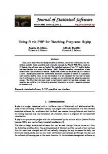
Journal of Statistical Software September 2008, Volume 28, Issue 1.

http://www.jstatsoft.org/

Computing and Displaying Isosurfaces in R Dai Feng

Luke Tierney

University of Iowa

University of Iowa

Abstract This paper presents R utilities for computing and displaying isosurfaces, or threedimensional contour surfaces, from a three-dimensional array of function values. A version of the marching cubes algorithm that takes into account face and internal ambiguities is used to compute the isosurfaces. Vectorization is used to ensure adequate performance using only R code. Examples are presented showing contours of theoretical densities, density estimates, and medical imaging data. Rendering can use the rgl package or standard or grid graphics, and a set of tools for representing and rendering surfaces using standard or grid graphics is presented.

Keywords: marching cubes algorithm, density estimation, medical imaging, surface illumination, shading.

1. Introduction Isosurfaces, or three-dimensional contours, are a very useful tool for visualizing volume data, such as data in medical imaging, meteorology, and geoscience. They are also useful for visualizing functions of three variables, such as fitted response surfaces, density estimates, or other density functions. The function contour3d, available in the R (R Development Core Team 2008) package misc3d (Feng and Tierney 2008), uses the marching cubes algorithm (Lorensen and Cline 1987) to compute a triangular mesh approximating the contour surface and renders this mesh using either the rgl (Adler and Murdoch 2008) package or standard or grid graphics. Several approaches are available for rendering multiple contours, including alpha blending for partial transparency and cutaway views. The next section presents several examples illustrating the use of contour3d. The third section describes the particular version of the marching cubes algorithm used, and some computational issues. The fourth section presents utilities for representing surfaces and for rendering surfaces using standard or grid graphics. The final section presents some discussion

2

Computing and Displaying Isosurfaces in R

(a) Epicenter locations

(b) Locations with density contour

Figure 1: Locations of earthquake epicenters rendered using rgl. and directions for future work.

2. Examples The data set quakes included in the standard R distribution includes locations of epicenters of 1000 earthquakes recorded in a period since 1964 in a region near Fiji. Figure 1a shows a scatterplot of the locations. Figure 1b adds a contour of a 3D kernel density estimate, which helps to reveal the geometrical structure of the data. The scatterplot is created using R> R> R> R>

library("rgl") points3d(quakes$long/22, quakes$lat/28, -quakes$depth/640, size = 2) box3d(col = "gray") title3d(xlab = "long", ylab = "lat", zlab = "depth")

The kernel density estimate is computed using the function kde3d in package misc3d and rendered using contour3d and the default rgl rendering engine: R> de contour3d(de$d, level = exp(-12), x = de$x/22, y = de$y/28, z = de$z/640, + color = "green", color2 = "gray", add = TRUE) The d component of the result returned by kde3d is a three-dimensional array of estimated density values. The argument color is the color used for the side of the surface facing lower function values; color2 specifies the color for the side facing higher values, and defaults to the value of color. The color arguments can be an R color specification or a function of three arguments, the x, y, and z coordinates of the midpoints of the triangles. This can be used to color the triangles

Journal of Statistical Software

3

Figure 2: Density contour surface for variables Sepal.Length, Sepal.Width, and Petal.Length from the iris data set, with false color showing the levels of the fourth variable, Petal.Width, predicted by a loess fit.

individually, for example to use false color to encode additional information. Figure 2 shows a contour of a kernel density estimate of the marginal density of the variables Sepal.Length, Sepal.Width, and Petal.Length from the iris data (Anderson 1935). Color is used to encode the level of a loess fit of the fourth variable, Petal.Width, to the first three variables. This shows the positive correlation between Petal.Length and Petal.Width. The plot is created by evaluating the expressions R> R> + R> + + + + + R> R> R> +

de R> R>

5

n R> R>

library("AnalyzeFMRI") template α

Figure 9: Resolving face ambiguity

3.2. Computational considerations The core of the marching cubes algorithm is table-lookup. There are several tables in contour3d used to determine how an isosurface intersects each cube. For example, having 256 entries (each corresponding to one case), table Faces specifies which faces need to be checked to make further judgment on sub-cases. Table Edges shows, for each case, which edges are intersected by the isosurface. These tables are generated automatically based on basic configurations, their rotations, and switching of the positive and negative values. In order to match each cube with a table entry, the execution flow could be serial, using a loop to iterate through the cubes one-by-one. This approach, however, is not very efficient in pure R code, although a compiler might be able to improve this. Besides, R facilitates vectorization very well by functions such as ifelse, which and so on. One important prerequisite for vectorization is that there is no dependency between successive inputs and outputs. In order to vectorize the marching cubes algorithm, each operation is executed on all cubes (or cubes with the same properties) simultaneously on the condition that there is no dependency among cubes. For example, the determination on cases of each cube and vertices of triangles (the bilinear interpolation) can be vectorized under careful coding. Computation of the table lookup index values can also be vectorized if care is taken. For example, for basic case 6 there are face and internal ambiguities. Two logical variables, index1 and index2, are assigned for each ambiguity and a combined index is computed as index = index1 + 2 * index2.

4. Rendering surfaces in standard and grid graphics Surfaces, such as three dimensional contour surfaces or surfaces representing functions of two variables, can be rendered by approximating the surfaces by a triangular mesh and passing the mesh on to a rendering function. The facilities provided by the rgl package are very well suited for interactive rendering and exploration, and can be used to generate snapshots as PNG images for inclusion in documents. At times it can also be useful to render triangle mesh surfaces using R’s standard or grid graphics systems (Murrell 2005). Rendering in standard and grid graphics can be done by drawing the triangles in back to front order. The three-

12

Computing and Displaying Isosurfaces in R

Case 0

Case 1

Case 2

Case 3.1

Case 3.2

Case 4.1.1

Case 4.1.2

Case 5

Case 6.1.1

Case 6.1.2

Case 6.2

Case 7.1

Case 7.2

Case 7.3

Case 7.4.1

Case 7.4.2

Case 8

Case 9

Case 10

Case 10.1.2

Case 10.2

Case 11

Case 12.1.1

Case 12.1.2

Case 12.2

Case 12.3

Case 13.1

Case 13.2

Case 13.3

Case 13.4

Case 13.5.1

Case 13.5.2

Case 14

Figure 10: The lookup table of the marching cubes 33 algorithm

dimensional structure is brought out by adjusting the colors of the triangles according to a simple lighting model based on the direction of the triangle’s surface normal vector relative to the position of the viewer and a lighting source. This section briefly describes the triangle data structure used in package misc3d and presents the some details of the rendering method along with some illustrative examples.

Journal of Statistical Software

13

4.1. Triangular mesh surfaces The triangle mesh data structure contains information representing the triangles, along with characteristics of the individual triangles and the surface as a whole that are used in rendering. The current representation is as a list object with the S3 class Triangles3D. For a mesh consisting of n triangles this structure currently includes components v1, v2, and v3, which are n × 3 matrices containing the coordinates of the vertices of the triangles. A more compact representation that takes into account the sharing of vertices is possible but not currently used. Properties specified in the structure include color and color2 for the color of the two sides of the triangles, alpha for the transparency level, fill indicating whether the triangles are to be filled, and col.mesh for the color of triangle edges. A final property, smooth, indicates whether shading is to be used to give the surface a smoother appearance. The color fields can contain a single color specification, a vector containing a separate color for each triangle, or a vectorized function used to compute the colors based on the coordinates of the triangle centers. color represents the color for the side for which the vertices in v1, v2, and v3 appear in clockwise order. The smooth property is a non-negative integer value. For the standard and grid engines it specifies the level of shading to be used as described below in Section 4.2. For the rgl engine a positive value indicates that vertex normal vectors should be computed and passed to the trinangles3d rendering function. Several functions are available for creating and manipulating triangle mesh objects. The functions contour3d and parametric3d create and optionally render contour surfaces and surfaces in three dimensions represented by a function of two parameters, respectively. The function surfaceTriangles creates a triangle mesh representation of a surface described by values over a rectangular grid. The constructor function makeTriangles creates a triangle mesh data structure from vertex specifications and property arguments. updateTriangles can be used to modify triangle properties, and scaleTriangles and translateTriangles to adjust the mesh itself.

4.2. Rendering triangular mesh surfaces Triangle mesh scenes are rendered by the function drawScene. This function performs the specified viewing transformation, computes colors based on a lighting model, possibly adding shading, performs a perspective transformation if requested, and passes the resulting modified scene on to the internal renderScene function. renderScene in turn merges the triangles into a single triangle mesh structure, optionally adds depth cuing, determines the z order of the triangles based on the triangle centers, and draws the triangles from back to front using the appropriate routine for drawing filled polygons using standard or grid graphics. The following subsections describe the lighting, shading, and depth cuing steps in more detail.

Illumination Local illumination models (also called lighting or reflection models) provide a means of showing three dimensional structure in a two dimensional view by modeling the way in which light is reflected towards the viewer from a particular point on a surface. Simple models used in computer graphics usually consider two forms of light, ambient light with intensity Ia and light from one or more point light sources with intensity Ii , and two forms of reflection, diffuse

14

Computing and Displaying Isosurfaces in R

N H L

R V θ

θ

Figure 11: Vectors used in the reflection model. L is the direction to the light source, V is the direction to the viewer, and N is the surface normal. R is the reflection vector and H is the half-way vector proportional to (L + V )/2. and specular. The light intensity seen by the viewer IV is the sum of the intensities of an ambient component IV a , a diffuse component IV d , and a specular component IV s . Separate intensities are used for the red, green, and blue channels but this is suppressed in the following discussion. The description given here is based mainly on Foley, van Dam, Feiner, and Hughes (1990, Section 16.1). Ambient light represents a diffuse, non-directional source of light that illuminates all surfaces equally. The ambient component seen by the viewer is usually represented as IV a = Ia ka Oa where ka is an ambient reflection coefficient associated with the object being rendered and Oa represents the object’s ambient color. Diffuse or Lambertian reflection reflects light from a point source equally in all directions away from the surface. The intensity of light from source i reflected towards the viewer is determined by the angle between the unit vector Li in the direction of the light source and the unit normal vector N at the point of interest on the surface. The intensity of light from a single light source is Ii kd Od cos(θLi ,N ) = Ii kd Od (Li · N ) where kd is the diffuse reflection coefficient associated with the object and Od is the object’s diffuse color. The intensity of diffuse light seen by the viewer is thus X IV d = Ii kd Od (Li · N ) i

Specular reflection is the reflection of light off a shiny object. An ideal reflector reflects this light only in the direction of the reflection unit vector R, shown in Figure 11, and the color of

Journal of Statistical Software ambient diffuse specular exponent sr

15

ambient reflection coefficient ka diffuse reflection coefficient kd specular reflection coefficient ks specular exponent n contribution of object color to specular color

Table 1: Components of a material structure

ambient diffuse specular exponent sr

metal 0.45 0.45 1.50 25 0.50

shiny 0.36 0.72 1.08 20 0

dull 0.3 0.8 0 10 0

default 0.3 0.7 0.1 10 0

Table 2: Some pre-defined materials. the reflected light matches the color of the light source. The Phong model (Bui-Tuong 1975) is a commonly used model for imperfect reflectors that represents the intensity of specularly reflected light seen by the viewer as a smooth function of the angle between the reflection vector R and a unit vector V in the direction of the viewer. This angle is twice the angle between the surface normal and the half-way vector Hi proportional to (Li + V )/2, which is easier to compute. The specific version we have used represents the intensity of light from a single source specularly reflected towards the viewer as Ii ks Os cosn (θHi ,N ) = Ii ks Os (Hi · N )n where ks is the specular reflection coefficient of the object, Os is the object’s specular color, and n is called the specular reflection exponent. For a perfect reflector the specular color is identical to the light color and the exponent is infinite. The total specular contribution is X

Ii ks Os (Hi · N )n

i

We use a simplified version of the model just described: Only a single white point light source is supported, and ambient light is white with the same intensity as the point light source. The ambient and diffuse object colors are assumed to the identical, and the specular object color is assumed to be a convex combination of the diffuse object color and white. The material characteristics are collected into a material structure with components listed in Table 1. Several materials are pre-defined, with characteristics based loosely on those found in MATLAB (The MathWorks, Inc. 2007); these are shown in Table 2. Rendering functions take a material argument that can be a character string naming a pre-defined material type or a list of the required components. Figure 12 shows a contour surface of a kernel density estimate from three variables of the iris data set rendered using the four pre-defined materials. The figure is created by

16

Computing and Displaying Isosurfaces in R

Figure 12: Contour surface of kernel density estimate for the first three variables in the iris data set rendered using the four standard material settings.

R> xlim ylim zlim de opar for (m in c("default", "dull", "metal", "shiny")) { + contour3d(de$d, 0.1, de$x, de$y, de$z,color = "lightblue", + engine = "standard", material = m) + title(paste('material = "', m, '"', sep = "")) + } par(opar)

Journal of Statistical Software

(a) no shading

17

(b) shading with smooth = 2

Figure 13: Contour surface of kernel density estimate for the first three variables in the iris data set rendered using no additional shading and using two iterations of shading.

Shading A triangular mesh is usually used as an approximation to a smooth surface. Rendering with an illumination model renders the approximate surface and clearly shows the facets of the approximation. Shading uses color variations within a facet to create a smoother representation. These color variations are computed based on surface normals. Suppose we have surface normals at each of the vertices of a facet. These may be available analytically or can be approximated by averaging the normals of the facets that share the vertex. One approach, known as Gouraud shading or intensity interpolation shading, computes colors for each vertex based on a lighting model and the vertex normals, and linearly interpolates colors across the facet. A second approach, Phong shading or normal vector interpolation shading, computes an interpolated normal vector for points within a facet and uses the interpolated normal vector to determine an appropriate color for the point. Shading models are usually used at the pixel level, and often implemented in hardware. rgl uses this approach via the underlying OpenGL library. As a simple, though computationally costly, alternative for standard and grid graphics we can divide each triangle into four subtriangles by splitting each edge in the middle, and apply either shading algorithm to the sub-triangles. This process can in principle be iterated several times. The smooth argument to drawScene specifies one plus the number of times to divide the triangles and uses the Phong shading model to compute appropriate colors. For smooth = 1 there is no sub-division: the vertex normals are computed by averaging the triangle normals for triangles sharing the vertex, and a new surface normal for each triangle is then computed by interpolation of its vertex normals. Figure 13 shows the density estimate contour surface for the iris data rendered with no shading and with smooth = 2 corresponding to one level of subdivision. The figure is created with

18

Computing and Displaying Isosurfaces in R

R> opar contour3d(de$d, 0.1, de$x, de$y, de$z, color = "lightblue", + engine = "standard", smooth = 0) R> contour3d(de$d, 0.1, de$x, de$y, de$z, color = "lightblue", + engine = "standard", smooth = 2) par(opar) Aside from the higher cost in computing time and memory usage, using too high a level of smooth can cause the rendering quality to deteriorate as a result of artifacts due to the use of polygon filling for rendering the result. This may be exacerbated on devices that use anti-aliasing.

Atmospheric attenuation Simulated atmospheric attenuation can be used as a form of depth cuing to help indicate which parts of a scene are closer to the viewer and which are farther away. This approach blends the colors of more distant objects with the background color. The argument depth to the function drawScene specifies whether this form of depth cuing is to be used; if depth is non-zero then the rendering code computes the z values and maximal z value zmax for the scene and sets 1 + depth × z s= 1 + zmax Then the color intensities I are modified to sI + (1 − s)Ibg where Ibg represents the intensity of the background color. Figure 14 illustrates depth cuing by simulated atmospheric attenuation using the elevation data for the Maunga Whau volcano included in the R distribution. Figure 14a uses no depth cuing and Figure 14b uses depth=0.3. The code to create the figures is

(a) no depth cuing

(b) with depth cuing

Figure 14: Surface plot of the Maunga Whau volcano with and without depth cuing and using smooth = 3 level shading.

Journal of Statistical Software R> R> R> R> + + + + R> R> + R> + + R>

19

z +

xlim