is free to perform an arbitrary additional number of internal steps). Computing ...... probabilistic settings like CCS and Ï-calculus [39,40] or in the other probabilistic models, as ... probability such that n â N, s1 R tj for 0 < j ⤠n, and u1 R u2. ...... [52] Stewart, W.J.: Introduction to the Numerical Solution of Markov Chains. Prince ...
Computing Behavioral Relations for Probabilistic Concurrent Systems Daniel Gebler1 , Vahid Hashemi2,3 , and Andrea Turrini4 1
Department of Computer Science, VU University Amsterdam, De Boelelaan 1081a, NL-1081 HV Amsterdam, The Netherlands 2
Max Planck Institute for Informatics, 66123 Saarbr¨ ucken, Germany 3
Department of Computer Science Saarland University, 66123 Saarbr¨ ucken, Germany 4
State Key Laboratory of Computer Science, Institute of Software, Chinese Academy of Sciences, 100190 Beijing, China
Abstract. Behavioral equivalences and preorders are fundamental notions to formalize indistinguishability of transition systems and provide means to abstraction and refinement. We survey a collection of models used to represent concurrent probabilistic real systems, the behavioral equivalences and preorders they are equipped with and the corresponding decision algorithms. These algorithms follow the standard refinement approach and they improve their complexity by taking advantage of the efficient algorithms developed in the optimization community to solve optimization and flow problems.
1 1.1
Introduction Probabilistic Systems
Probability, time, and nondeterminism. These are three main characteristics of several real-world applications. Probability occurs every time the behavior of the applications is not unique, either by construction or by physical properties. For example, distributed algorithms like the Zeroconf protocol or cryptographic protocols like SSL are based on random choices to break symmetry or to insert uncertainty in order to achieve their goals. Each time a message is transmitted on the network, in fact, transmission protocols have to manage the corruption of the messages, as well as their loss, as the effect of the interference with other concurrent transmissions or physical properties of the transmission medium. For instance, simultaneous transmissions on the same channel of a wireless network lead to the collision of the sent messages and their corruption. Beside probabilities, these systems often have another source of uncertainty, namely nondeterminism, that appears whenever an event may occur with unpredictable behavior; for instance, the event of a host starting the transmission in a wireless network.
Time governs the evolution of the system: with the time passing, the system performs and reacts to actions and correspondingly changes its state, according to its goals. Time can be considered as a discrete component (e.g., a program running on a computer performs one operation at each tick of the digital clock) or as a continuum behavior (e.g., the arrival and service of customers at the information desk). To study the properties of such real-world applications, several models have been proposed by researchers: the basic model in the discrete time domain is the discrete time Markov chains (DTMCs) model [26, 52], where the time is discrete (i.e., the system performs one operation per clock tick) and only probability determines the reached states. The continuous-time counterpart is known as the continuous-time Markov chains (CTMCs) [3, 5] model, where exponentially distributed sojourn times distributions control the evolution of the system. DTMCs and CTMCs are purely probabilistic, and they have been extended with nondeterminism to permit different operations or behaviors from a specific state. This extension results to Markov decision processes (MDPs) [10,31,32,44] and continuous-time Markov decision processes (CTMDPs) [7, 11, 31, 44, 54], respectively. These models, despite being widely used to represent and study real systems, are not fully compositional, that is, there is no guarantee that complex systems can be obtained by composing smaller components while preserving the intended behavior. This property is rather important as it is usually much easier to model and study (a set of) small systems and then combine them together rather than a single large system. Moreover, in the real world, usually applications and protocols involve several parties each one composed by modules working together in parallel. Two models have been proposed to achieve such compositional property: the probabilistic automata (PAs) model [47, 48] for discrete time systems and the interactive Markov chains (IMCs) [28] model for continuous-time systems. Recently one model has been proposed to unify and merge all such models in a single framework: the Markov automata (MAs) model [17, 22, 23]. This formalism is suitable for studying systems featuring continuous-time based behaviors as well as probabilistic and nondeterministic choices. Moreover, the Markov automata model provides the semantics to every generalized stochastic Petri net (GSPN) [19], a popular modelling formalism for performance and dependability analysis. 1.2
Comparing System Behaviors
Given a real world system we want to analyze, for instance by verifying whether it satisfies a set of properties, we can model it in several ways. This analysis is commonly known as model checking. In particular, we can decide to model it as a DTMC or as a PA whenever we are interested in its properties as a discrete time system; alternatively, if we want to study its behavior in continuous time, we can use CTMCs or IMCs. The choice of the model framework depends on the properties we are interested in and the details we want to consider. Once the model framework has been chosen, the real system can be represented by several different models: for example, we can use different names for
the states, we can encode probabilistic choices as sequences of events or as single events, we can detail or abstract from particular details, and so on. It is clear that these choices affect the resulting model whose size may vary even if all these models represent the same real system. A possible way to abstract away from this modelling details is to use the so called simulation and bisimulation relations that allow us to declare that two models are similar or equivalent whenever they are related, respectively. Intuitively, a system S1 simulates a system S2 if S1 is able to mimic whatever S2 can do; the bisimulation requires that also S2 simulates S1 . Usually, a simulation (or bisimulation) is defined as a binary relation over the states of the model and for each pair (s1 , s2 ), if s1 can perform a step, then s2 has to match such step via its own steps in order to reach states that are related to the states reached from s1 . Depending on the steps s2 is allowed to perform, simulation relations can be classified as strong (s2 has to match with exactly one step) or as weak (s2 is free to perform an arbitrary additional number of internal steps). Computing such simulation relations is rather easy by using classical refinement algorithms, provided that we have a procedure for deciding the existence of the matching step from s2 given a step from s1 . As we will see in Section 6, such procedure is the only part that has to be changed in order to decide different simulations and it is also the bottleneck of the computation and the main source of the complexity of the decision procedure. We are interested in systems related by a simulation relation since also the properties they satisfy are related, so we can check whether the real world system satisfies a given property by verifying it in one of the similar models: the theory ensures us that the evaluation of the property does not depend on the specific model we consider to represent the real world system. When we consider the bisimulation relation, among all possible bisimilar models there is a unique minimal model (up to isomorphism) that represents the original system [21]: the quotient model. The quotient is the model with the minimum number of states and transitions still behaving as the system we want to analyze; this minimality mitigates the state explosion problem of the model checking [8, 14, 34] as well as it helps in reducing the computational effort needed to verify whether the desired properties are fulfilled. Moreover, the computation of the quotient automaton is independent on the properties we want to check, thus even if it may be rather time consuming, the overall gain it provides to the following model checking phase may justify it. 1.3
Optimization Problems
Optimization or mathematical programming uses mathematical techniques to find the best solution among a set of given alternatives. More precisely, an optimization problem asks for maximizing or minimizing a real valued function for which the variables take values from a permissible set. It includes many diverse areas such as decision theory [42], flow network optimization [1] and so on. Flow network optimization is a subclass of linear programming that has application
in a number of domains such as computer science, logistics, transportation systems. Although flow network based models are not as wide as models that can be formulated mathematically using linear or integer programming, they can be solved very quickly which enables them to be a powerful tool for decision making [1]. 1.4
Probabilistic Systems vs. Optimization
To a casual observer, flow and optimization problems seem rather unrelated to probabilistic concurrent systems. In fact, as we have seen, the former aim to optimize problems like resource allocation or goods transportation and distribution while the latter model systems that run in parallel where the behavior depends on probabilistic events as well like random failures, errors, and choices needed to break symmetry. To a careful observer, flow and optimization problems and probabilistic concurrent systems are not so unrelated, since the probability mass concentrated in the initial state can be seen as a liquid that flows and distributes in the network representing the possible evolution of the system. To highlight this connection, in this survey we consider a selection of papers [29,30,55,57] that, together with other works in concurrency literature such as [2,4,13,15,20,21,43,45], make use of flow and optimization problems to decide or solve efficiently the challenges of probabilistic concurrent systems. Organization of the paper. After the mathematical preliminaries in Section 2, we present in Section 3 the discrete and continuous-time models, followed in Section 4 by the simulation and bisimulation relations defined on them. We recall in Section 5 the theory about networks and flow problems that are widely used in Section 6 to efficiently compute simulations and bisimulations. We conclude the paper in Section 7.
2 2.1
Mathematical Preliminaries Functions and Relations
Given a set X and ⊥ ∈ / X, we denote by X⊥ the set X ∪ {⊥}. Let X, Y be two finite sets, f : X → R and g : X × YP→ R be two functions. 0 0 For X 0 ⊆ X, we denote by P f (X ) the value f (X ) = x∈X 0 f (x); for 0x ∈ X 0 0 and Y ⊆ YP , g(x, Y ) = y∈Y 0 g(x, y) and similarly, for y ∈ Y and X ⊆ X, g(X 0 , y) = x∈X 0 g(x, y). Finally, we define for each x ∈ X and y ∈ Y the functions g(x, · ) : Y → R and g( · , y) : X → R as g(x, · )(y 0 ) = g(x, y 0 ) for each y 0 ∈ Y and g( · , y)(x0 ) = g(x0 , y) for each x0 ∈ X, respectively. Given two functions f, g : X → R and p ∈ R, we denote by p · f : X → R the function (p · f )(x) = p · f (x) for each x ∈ X and f + g : X → R the function (f + g)(x) = f (x) + g(x) for each x ∈ X. For a function f : X → R≥0 , we denote by Supp(f ) the support set Supp(f ) = { x ∈ X | f (x) > 0 }.
Given a relation R ⊆ X × Y and the sets X 0 ⊆ X and Y 0 ⊆ Y , we define R(X 0 ) = { y ∈ Y | ∃x ∈ X 0 .x R y } and R−1 (Y 0 ) = { x ∈ X | ∃y ∈ Y 0 .x R y }. Given a relation R ⊆ X × X, we call R ∩ R−1 the kernel of R and we denote by R⊥ ⊆ X⊥ × X⊥ the relation R ∪ { (⊥, x) | x ∈ X⊥ }. 2.2
Probability Distributions
For a set X, denote by Disc(X) the set of discrete probability distributions over X, and by SubDisc(X) the set of discrete sub-probability distributions over X. Since a discrete sub-probability distribution ρ ∈ SubDisc(X) can be seen as a function ρ : X → [0, 1], we adopt the same terminology and operations. Given ρ ∈ SubDisc(X), we denote by ρ(⊥) the value 1 − ρ(X) where ⊥ ∈ / X, and by |ρ| the size |Supp(ρ)|. We extend ρ to a probability distribution ρ⊥ ∈ Disc(X⊥ ) by defining ρ⊥ (⊥) = 1 − ρ(X) and ρ⊥ (x) = ρ(x) for each x ∈ X. We denote by δx , where x ∈ X⊥ , the Dirac distribution such that δx (y) = 1 for y = x, 0 otherwise. For a sub-probability distribution ρ, we also write ρ = { (x, px ) | x ∈ X } where px is the probability of x. We say that ρ is stochastic if ρ(X) = 1 and absorbing if ρ(⊥) = δ⊥ . We sometimes refer to ρ(X) as the mass of ρ. The lifting L(R) ⊆ Disc(X) × Disc(X) [34] of a relation R ⊆ X × X to distributions is defined as: for ρ1 , ρ2 ∈ Disc(X), ρ1 L(R) ρ2 holds if there exists a weighting function w : X × X → [0, 1] such that 1. for each (x1 , x2 ) ∈ X × X, w(x1 , x2 ) > 0 implies x1 R x2 , 2. for each x1 ∈ X, w(x1 , X) = ρ1 (x1 ), and 3. for each x2 ∈ X, w(X, x2 ) = ρ2 (x2 ). This definition of lifting has been proposed for discrete systems [34, 50] and it is indeed equivalent [55] to the definition based on R-closure introduced by [18] for non-discrete systems: the lifting L(R) ⊆ Disc(X) × Disc(X) of a relation R ⊆ X × X is defined as: for ρ1 , ρ2 ∈ Disc(X), ρ1 L(R) ρ2 holds if for each X 0 ⊆ X, ρ1 (X 0 ) ≤ ρ2 (R(X 0 )). Extending the lifting to sub-distributions is rather easy [57]: for ρ1 , ρ2 ∈ SubDisc(X), ρ1 L(R) ρ2 holds if there exists a weighting function w : X⊥ ×X⊥ → [0, 1] such that 1. for each (x1 , x2 ) ∈ X⊥ × X⊥ , w(x1 , x2 ) > 0 implies x1 R⊥ x2 , 2. for each x ∈ X⊥ , w(x, X⊥ ) = ρ1 (x), and 3. for each x ∈ X⊥ , w(X⊥ , x) = ρ2 (x).
3
The Models
We now introduce the formal models for probabilistic concurrent systems we consider in this survey paper. We first recall the discrete time models and then the continuous-time models. In this work we consider only finite models, i.e., systems such that states, actions, and transition relations are finite.
3.1
Discrete Time Models
The first model we consider is the labelled substochastic discrete time Markov chain model where each state enables only a transition that may reach several states, each one with a given probability. The status of the system is represented by a set AP of atomic propositions that are true in the given state. Definition 1 (Substochastic discrete time Markov chain [8, 33]). A labelled substochastic Discrete Time Markov Chain (sDTMC) S is a tuple S = (S, s¯, P, L) where S is a finite set of states, s¯ is the start state, P : S ×S → [0, 1] is a probability matrix such that P(s, · ) ∈ SubDisc(S) for all s ∈ S, and L : S → 2AP is a labeling function. Given a state s and the associated distribution µs = P(s, · ) ∈ SubDisc(S), we call (s, µs ) a transition and we say that (s, µs ) is enabled by s and that µs is the target of (s, µs ). 1 2
s
3 10
3 10 1 2
1 2
t
3 10
u
v
3 10
Figure 1: An example of substochastic discrete time Markov chain
Figure 1 shows an example of a sDTMC, where s is the initial state, denoted by the short incoming arrow. For each state, we represent the enabled transition by a set of arrows grouped by an arc and pointing to the target states, each one decorated with the corresponding probability. For example, the transition 3 enabled by s reaches t and u with probability 21 and 10 , respectively. As usual in this kind of representation of the model, to keep the picture clear we have omitted the arrows reaching states with probability 0. For instance, from s there should be also an arrow reaching v with probability 0. As labels of the states, we take AP = S = {s, t, u, v} and we let L(z) = z for each state z ∈ S. Note that the transitions from both s and u have as target a sub-probability distribution that is not a probability distribution. In fact, for the transition (s, µs ) the mass 8 9 of µs is 10 and the transition (u, µu ) the mass of µu is 10 . We call a state s stochastic (absorbing) if the distribution P(s, · ) is stochastic (absorbing) respectively. For the sDTMC in Figure 1, t is stochastic, v is absorbing while both s and u are neither stochastic nor absorbing. If we restrict the states of a sDTMC to be either stochastic or absorbing, we obtain a discrete time Markov chain:
Definition 2 (Discrete time Markov chain [26, 52]). A labelled Discrete Time Markov Chain (DTMC) D is a labelled sDTMC D = (S, s¯, P, L) such that for each state s ∈ S, P(s, S) ∈ {0, 1}.
1 2
s
1 3
1 3 1 2
5 8
t
3 8
u
v
1 3
Figure 2: An example of discrete time Markov chain
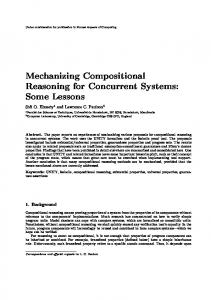
Figure 2 shows an example of a DTMC. It is actually the sDTMC in Figure 1 where probability distributions have been normalized to have mass 1. These two models are suitable for systems exhibiting only probabilistic behaviors, that is, they are not able to represent systems where different transitions are available from the states. For instance, the system that is in a particular state may react differently to different stimuli and this can be modeled by performing different transitions leading to different distributions over the states of the system. We call this capacity nondeterminism that is encoded, together with probability, by the following two discrete time models: Markov decision processes and probabilistic automata. In order to have a uniform approach, for probabilistic automata we adopt the notation of [57] instead of the one used in [47, 48]. Definition 3 (Probabilistic automaton [47, 48]). A Probabilistic Automaton (PA) P is a tuple P = (S, s¯, Σ, →, L) where S is a finite set of states, s¯ is the start state, Σ is a finite set of actions, → ⊆ S × Σ × Disc(S) is a finite probabilistic transition relation, and L : S → 2AP is a labeling function. The set Σ is divided in two sets H and E of internal (hidden) and external actions, respectively. We remark that the definition of probabilistic automata we are presenting here is different from the original one given by Segala in [48] named simple probabilistic automata, but currently known as just probabilistic automata. In fact, in such work (simple) probabilistic automata are defined as follows (cf. [48, Section 3.1]): A Probabilistic Automaton (PA) P is a tuple (S, s¯, Σ, →) where S is a countable set of states, s¯ ∈ S is the start state, Σ is a countable set of actions, and → ⊆ S × Σ × Disc(S) is a probabilistic transition relation. The main difference with Definition 3 is that in [48] there is no labeling function. This difference can be easily bridged by defining L as L(s) = ∅ for each s ∈ S. Figure 3 shows an example of a PA where H = {τ } and E = {a, b}. In a probabilistic automaton P we can distinguish between two kinds of nondeterminism: external and internal nondeterminism. We say that a state s
1 1 2
s
a
a
1 2
b τ
1 2
1 2 3 8
5 8
t 1
b
u
1 1
b
v
a
Figure 3: An example of probabilistic automaton
exhibits external nondeterminism if there exist two different actions a and b such that (s, a, µa ) ∈ → and (s, b, µb ) ∈ → for some µa , µb ∈ Disc(S). For instance, this is the case for the state v of the PA in Figure 3 since we have the two transitions (v, a, δs ) and (v, b, δu ). On the other hand, we say that a state s exhibits internal nondeterminism if there exist an action a and two different distributions µ1 , µ2 ∈ Disc(S) such that (s, a, µ1 ) ∈ → and (s, a, µ2 ) ∈ →. This happens for the state u that enables two different transitions both with action b. Note that a state may exhibit both internal and external nondeterminism (as happens for v) or none of them (see states s and t). 3.2
Continuous-Time Models
We now consider the continuous-time counterparts of the previous models, where state transitions are governed by the passing of the time. Essentially, they are defined as the discrete time models except for the probability distributions that are replaced by transition rates, i.e., the speed of transition firing. The first model we recall is about continuous-time Markov chains that are just discrete time Markov chains where the probability matrix is replaced by the rate matrix. Definition 4 (Continuous-time Markov chain [5, 44, 55]). A labelled Continuous-Time Markov Chain (CTMC) C is a tuple C = (S, s¯, R, L) such that S, s¯, and L are defined as for DTMC and R : S × S → R≥0 is the rate matrix. Note that the usual definition of CTMCs, such as the one in [3], requires that R : S × S →PR where for each s ∈ S, R(s, s0 ) ≥ 0 for each s0 6= s and R(s, s) = − s0 6=s R(s, s0 ). As remarked in [5], allowing self loops neither alters the transient nor the steady-state behavior of the CTMC, but it allows the usual interpretation of the linear-time CSL operators like next-step and until. Figure 4 shows an example of a CTMC. Greek letters λ, κ, and ρ are the rates governing the speed of the firing of the transitions. So, for example, the λ on the transition from s to t means that R(s, t) = λ. We omitted the transitions with rate 0 to keep the picture clear. The probability of performing a transition and reaching a given state can be computed as follows: starting from the state s, the probability of performing a
λ
s
λ
κ
λ
t
ρ
u
v
κ
Figure 4: An example of continuous-time Markov chain transition within time t is 1 − e−R(s,S)·t and the probability of reaching the state 0 ) s0 with this transition is (1 − e−R(s,S)·t ) · R(s,s R(s,S) . This allows us to consider the DTMC embedded into a CTMC that captures the system behavior after abstracting away the time: Definition 5 (Embedded DTMC [5, 55, 57]). Let C be a CTMC. The embedded DTMC D of C is defined by emb(C) = (S, s¯, P, L) where for each s, s0 ∈ 0 ) 0 S, P(s, s0 ) is defined as P(s, s0 ) = R(s,s R(s,S) if R(s, S) > 0, and P(s, s ) = 0 otherwise. Similarly to CTMCs and DTMCs, the continuous-time counterparts of PAs, called continuous-time probabilistic automata (CTPA), are obtained by replacing the transition relation with a rate matrix. We call a function r : S → R≥0 a rate function and we denote the set of all rate functions by Rate(S). Given the rate function r, we call r(S) the exit rate. Given R and a state s of a CTMC C, we call R(s, · ) : S → R≥0 the rate function associated with s and we usually denote it by rs . Definition 6 (Continuous-time probabilistic automaton [11, 37, 44]). A Continuous Time Probabilistic Automaton (CTPA) CP is a tuple CP = (S, s¯, Σ, R, L), where S is a finite set of states, s¯ is the start state, Σ is a finite set of actions, R ⊆ S × Σ × Rate(S) is a finite rate matrix, and L : S → 2AP is a labeling function.
λ
s
λ c
b a
a a
a σ
κ
λ
t κ
θ
u
c
ρ
v
a
Figure 5: An example of continuous-time probabilistic automaton
Figure 5 shows an example of CTPA; arrows emanating from a state with the same label and shape belong to the same transition. For instance, state s enables
two transitions (s, a, r) and (s, a, r0 ) with r, r0 ∈ Rate(S) such that r(t) = σ, r(u) = θ, and r(s) = r(v) = 0 and r0 (t) = λ, r0 (u) = κ, and r0 (s) = r0 (v) = 0, respectively. 3.3
Mixed Discrete and Continuous-Time Models
We now present two models that merge continuous-time and discrete time behavior, the interactive Markov chains and the Markov automata. They exhibit continuous-time behavior like CTMCs, where transitions are fired by the passage of the time, as well as discrete time behavior like labelled transitions systems where transitions are fired by actions. These two models are especially suited for compositional reasoning over continuous-timed systems due to the separation of action and Markovian transitions and the maximal progress assumption, that is, if a state enables both timed transitions and internally labelled transitions, then the latter take precedence and the former are ignored. Definition 7 (Markov automaton [17,22,23]). A Markov Automaton (MA) MA is a tuple MA = (S, s¯, Σ, →, R, L) where S is a finite set of states, s¯ is the start state, Σ is a finite set of actions, → ⊆ S × Σ × Disc(S) is a finite probabilistic transition relation, R ⊆ S × R≥0 × S is a finite set of timed transitions, and L : S → 2AP is a labeling function. 1 1 2
a
s
a
1 2
b τ
1 2
5 8
t λ
1 2 3 8
u
v
κ 1
a
Figure 6: An example of Markov automaton
Figure 6 shows an example of a MA. As for the CTMC in Figure 4, we use Greek letters λ and κ for the rates governing the speed of the firing of the transitions that we represent by dashed arrows in order to distinguish them from probabilistic transitions. An interactive Markov chain is an MA such that each probabilistic transition leads to a Dirac distribution, i.e., to a single state: Definition 8 (Interactive Markov chain [28]). An Interactive Markov Chain (IMC) I is a tuple I = (S, s¯, Σ, →, R, L) where S is a finite set of states, s¯ is the start state, Σ is a finite set of actions, → ⊆ S × Σ × S is an interactive transition relation, R ⊆ S × R≥0 × S is a finite set of timed transitions, and L : S → 2AP is a labeling function.
a
s a
b τ
a
τ
b
u
t
v
κ
λ a
Figure 7: An example of interactive Markov chain
Figure 7 shows an example of an IMC. In particular, IMC can be seen as the merger of labelled transitions systems and CTMCs while MA can be seen as the merger of PAs and CTMCs. In fact, each model is an instance of the MA model with specific restrictions on → and R (cf. [22, Section 3]). As for probabilistic automata, the original definitions do not involve the labeling function L that we have added for uniformity. Again, the original model can be recovered by defining L(s) = ∅ for each s ∈ S.
3.4
Terminology and Notation
In the remaining of the paper we adopt the following terminology and notation, given in the context of probabilistic automata [27, 29, 47, 48, 57]. We refer to each instance of the discrete and continuous-time models as automaton and we denote it by A, that is, we use the term (discrete time) automaton and A for the sDTMC S, the DTMC D, and the PA P as well as the term (continuous-time) automaton and A for the CTMC C and the CTPA CP. Given a PA P, we let s,t,u,v, and their variants with indices range over S; a, b range over actions; and τ range over internal actions. A transition tr = (s, a, µ) ∈ a →, also denoted by s −→ µ, is said to leave from state s, to be labelled by a, and to lead to the target distribution µ, also denoted by µtr . We denote by src(tr ) the source state s and by act(tr ) the action a. We also say that s enables action a, that action a is enabled from s, and that (s, a, µ) is enabled from s. Finally, we let s −→ = { tr ∈ → | src(tr ) = s } be the set of transitions enabled by s and a → = { tr ∈ → | act(tr ) = a } be the set of transitions with label a. An execution fragment of a PA P is a finite or infinite sequence of alternating states and actions α = s0 a1 s1 a2 s2 . . . starting from a state s0 , also denoted by first(α), and, if the sequence is finite, ending with a state denoted by last(α), such that for each i > 0 there exists a transition (si−1 , ai , µi ) ∈ → such that µi (si ) > 0. The length of α, denoted by len(α), is the number of occurrences of actions in α. If α is infinite, then len(α) = ∞. Denote by frags(P) the set of execution fragments of P and by frags ∗ (P) the set of finite execution fragments of P. An execution fragment α is a prefix of an execution fragment α0 , denoted by α 6 α0 , if the sequence α is a prefix of the sequence α0 . The trace trace(α) of α is the sub-sequence of external actions of α; we denote by ε the empty trace and we define trace(a) = a for a ∈ E and trace(a) = ε for a ∈ H.
We extend the above terminology to the other models introduced so far, when applicable; in particular, we use → to denote the transition relations P and R of DTMCs and sDTMCs, and of CTMCs and CTPAs, respectively. For instance, given a DTMC D, a state s, and a probability distribution µ, we still τ call (s, τ, µ) a transition, denoted by s −→ µ, also written (s, τ, µ) ∈ P, provided that µ = P(s, · ). Note that here τ denotes just a step since it is not an actual action labeling the transition. Similarly, given a CTPA CP, a state s, an action a, and a rate function r, we still write (s, a, r) ∈ → if R(s, a) = r and we call a (s, a, r) a transition, denoted by s −→ r as well. For a CTPA CP and a rate function r, we denote by µr ∈ SubDisc(S) the induced sub-probability distribution defined by: if r(S) > 0, then for each s ∈ S, r(s) , and if r(S) = 0, then µr = δ⊥ . µr (s) = r(S) We adopt a similar notation also for CTMCs: for a CTMC C and a state s, we denote by µrs ∈ SubDisc(S) the sub-probability distribution induced by the rate function rs = R(s, · ), i.e., µrs = P(s, · ) for the embedded DTMC emb(C). Given an automaton A and a state s, we denote by post(s) the set of successors of the state s, that is, post(s) = Supp(P(s, · )) if A is a DTMC or a sDTMC, and post(s) = { s0 ∈ S | R(s, s0 ) > 0 } if A is a CTMC. For a sDTMC S and a state s, we denote by post ⊥ (s) the set post ⊥ (s) = Supp(µ⊥ ) where µ = P(s, · ). Similarly, we denote by pre(s) the set of predecessors of the state s, that is, pre(s) = { s0 ∈ S | P(s0 , s) > 0 } if A is a DTMC or a sDTMC, and pre(s) = { s0 ∈ S | R(s0 , s) > 0 } if A is a CTMC. Finally, we denote by reach(s) the states that are reachable with positive probability from s, that is, reach(s) = { t ∈ S | ∃α ∈ frags ∗ (A).last(α) = t }.
4
Simulations and Bisimulations
We recall now the main behavioral preorders and equivalences that are used for the models presented in Section 3. These relations allow us to relate system that are syntactically different, for instance because they use different names for the states, but exhibit equivalent behaviors. Moreover, they allow to reduce the size of the automata without changing their properties. This is especially useful to mitigate the state space explosion problem that usually happens in model checking [8, 14, 34]. An empirical investigation to show the effectiveness of such behavioral relations minimization is performed in [36]. This study indicates that for traditional model checking, huge state space reductions (up to logarithmic) may be acquired. It is worthwhile to mention that the definition of such relations is based on a single automaton; however, as we will see, they are usually used to relate two automata A1 and A2 . This technical problem is easily solved by taking the disjoint union of the two automata, that is, the automaton whose set of states is the disjoint union of the sets of states of A1 and A2 , and whose other components are the union of the corresponding components of A1 and A2 .
4.1
Strong Simulation and Bisimulation
The first relations we introduce are the strong simulation and bisimulation, that are the natural extension to probabilistic systems of the homonymous relations for labelled transition systems [39]. Definition 9 (Strong simulation for discrete time probabilistic automata [9, 50, 56, 57]). Let A be a discrete time probabilistic automaton. A relation R on S is a strong simulation if, for each pair of states s, t ∈ S such that s R t, – L(s) = L(t) and a – if s −→ µs for some probability distribution µs , then there exists µt such that a t −→ µt and µs L(R) µt . We say that the discrete time automaton A2 strongly simulates A1 if there exists a strong simulation R on the disjoint union S1 ] S2 such that s¯1 R s¯2 and we say that the state t strongly simulates the state s if there exists a strong simulation R such that s R t. We denote the coarsest strong simulation, called strong similarity, by .. In the remaining of the paper and similarly for the following simulations, we a refer to the second condition (if s −→ µs for some probability distribution µs , a then there exists µt such that t −→ µt and µs L(R) µt ) as the step condition since it ensures that from two similar states s and t, each transition (or step) from s is matched by a transition/step from t and the reached states are still related according to the lifting of the reached distributions. s1
s2
a
b
1 2
1 2
1 a
1 3
u1
t1 1
a 2 3
z1 1
A1
v1 1
a
b
1 3
2 3
1 a
1 3
2 3
u2
t2 1
b
b
a, b
v2 1 b
A2
Figure 8: Two PAs with L(x) = ∅ for each state x such that A1 . A2 . The single transition from u2 with action a, b is just a compact form for the two transitions (u2 , a, δu2 ) and (u2 , b, δu2 )
Figure 8 shows two probabilistic automata A1 and A2 such that A1 . A2 . In fact, consider the relation R = {(s1 , s2 ), (t1 , t2 ), (u1 , u2 ), (v1 , v2 ), (z1 , u2 )}; it is rather easy to verify that R satisfies Definition 9: it is trivial to verify the step condition for the pairs (t1 , t2 ), (u1 , u2 ), (v1 , v2 ), and (z1 , u2 ). The only interesting a case is the pair (s1 , s2 ); the transition s1 −→ µ1a with µ1a = {(t1 , 12 ), (u1 , 21 )} is a matched by s2 via the transition s2 −→ µ2a with µ2a = {(t2 , 13 ), (u2 , 23 )} such
that µ1a L(R) µ2a . The weighting function [34,56,57] wa justifying µ1a L(R) µ2a is defined as follows: 1 if x1 = t1 and x2 = t2 , 3 1 if x = t and x = u , 1 1 2 2 wa (x1 , x2 ) = 61 if x = u and x = u 1 1 2 2 , and 2 0 otherwise. b Similarly, the transition s1 −→ µ1b with µ1b = {(z1 , 31 ), (v1 , 32 )} is matched by s2 b via the transition s2 −→ µ2b with µ2b = {(u2 , 23 ), (v2 , 13 )} such that µ1b L(R) µ2b . The weighting function wb justifying µ1b L(R) µ2b is: 1 3 if x1 = z1 and x2 = u2 , 1 if x = v and x = u , 1 1 2 2 wb (x1 , x2 ) = 31 3 if x1 = v1 and x2 = v2 , and 0 otherwise.
The definition of strong simulation for continuous-time automata is almost the same, except for the fact that we require that t can move stochastically faster than s, i.e., t has a rate higher than s: Definition 10 (Strong simulation for continuous-time probabilistic automata [9, 56, 57]). Let A be a continuous-time probabilistic automaton. A relation R on S is a strong simulation if, for each pair of states s, t ∈ S such that s R t, – L(s) = L(t) and a – if s −→ rs for some rate function rs , then there exists a rate function rt such a that t −→ rt , µrs L(R) µrt , and rs (S) ≤ rt (S). We say that the continuous-time automaton A2 strongly simulates A1 if there exists a strong simulation R on the disjoint union S1 ] S2 such that s¯1 R s¯2 and we say that the state t strongly simulates the state s if there exists a strong simulation R such that s R t. We denote the coarsest strong simulation, called strong similarity, by .. Figure 9 shows two continuous time probabilistic automata A1 and A2 such that A1 . A2 . The relation R = {(s1 , s2 ), (t1 , t2 ), (u1 , u2 ), (t1 , u2 ), (u1 , t2 )} indeed justifies A1 . A2 : consider for instance the pair (t1 , t2 ); the rate function rt1 induces the probability distribution µrt1 = δu1 and the overall rate rt1 (S) = λ. For t2 , we have the rate function rt2 that induces the probability distribution µrt2 = δu2 and the overall rate rt1 (S) = 3λ, thus rt1 (S) ≤ rt2 (S). Since (u1 , u2 ) ∈ R, then δu1 L(R) δu2 is trivially satisfied, hence the step condition is satisfied. A similar argument shows that the step condition is satisfied for the pairs (u1 , u2 ), (t1 , u2 ), and (u1 , t2 ). Now, consider the pair (s1 , s2 ): we distinguish the case of the transitions with label b and c and the transition with label a, all from s1 . The transition from s1
s1
s2
2λ
c
c
b a
a
λ
a
λ
2λ
λ
u1
t1 2λ
4λ
b a
a
λ
a
3λ
3λ
4λ
u2
t2 3λ
a
A1
a
A2
Figure 9: Two CTPAs with L(s1 ) = L(s2 ) = {s} and L(x) = ∅ for each remaining state x such that A1 . A2
with label b induces the probability distribution µrsb = δt1 and the overall rate 1
rsb1 (S) = 2λ. For s2 , we have the rate function rsb2 that induces the probability distribution µrsb = δu2 and the overall rate rsb2 (S) = 4λ, thus rsb1 (S) ≤ rsb2 (S). 2 Since (t1 , u2 ) ∈ R, then δt1 L(R) δu2 trivially holds, hence the step condition is satisfied. The case for the label c is similar. The last step condition we have to check involves the transition with label a from s1 . The rate function rsa1 induces the probability distribution µrsa1 = λ a {(t1 , 3λ ), (u1 , 2λ 3λ )} and the overall rate rs1 (S) = 3λ. For s2 , we have the rate λ rsa2 that induces the probability distribution µrsa2 = {(t2 , 4λ ), (u2 , 3λ 4λ )} and the a a a overall rate rs2 (S) = 4λ. Obviously, rs1 (S) ≤ rs2 (S); µrsa L(R) µrsa is justified 1 2 by the weighting function w defined as 1 if x1 = t1 and x2 = t2 , 4 1 if x = t and x = u , 1 1 2 2 w(x1 , x2 ) = 12 32 if x = u and x = u 1 1 2 2 , and 0 otherwise The definition of strong bisimulation and strong bisimilarity, denoted by ∼, is obtained by requiring R to be a symmetric relation. Definition 11 (Strong bisimulation [38]). Let A be a discrete time or a continuous-time probabilistic automaton. A relation R on S is a strong bisimulation if R is symmetric and a strong simulation. We denote the coarsest strong bisimulation, called strong bisimilarity, by ∼. Other definitions of strong bisimulation require R to be an equivalence relation but it is easy to show that such definitions are equivalent to Definition 11. Finally, only strong bisimulation on IMCs has been defined [28], and it is the expected merge of the bisimulation for CTMCs and labelled transition systems: Definition 12 (Strong bisimulation for IMCs [28]). Let I be a IMC. An equivalence relation R on S is a strong bisimulation if, for each pair of states s, t ∈ S such that s R t,
– L(s) = L(t), a a – if s −→ s0 for some s0 ∈ S and a ∈ Σ, then there exists t0 such that t −→ t0 0 0 and s R t , and – if s does not enable a transition with label τ , then for each C ∈ S/R, γ(s, C) = P γ(t, C) where γ(v, C) = λ. λ { λ∈R≥0 |v −→v 0 ,v 0 ∈C } We say that the IMC A2 strongly bisimulates A1 if there exists a strong bisimulation R on the disjoint union S1 ] S2 such that s¯1 R s¯2 and we say that the state t strongly bisimulates the state s if there exists a strong bisimulation R such that s R t. We denote the coarsest strong bisimulation, called strong bisimilarity, by ∼. A simulation (and a bisimulation) can be seen as a game where in each round the challenger, or attacker, s proposes a transition, or step, that has to be matched by the defender t. The two states s and t are strong (bi-)similar if the defender is always able to match the challenging transitions proposed by the attacker, that is, the game can be played forever. 4.2
Strong Probabilistic Simulation and Bisimulation
The fact that (continuous-time) probabilistic automata may exhibit internal nondeterminism, i.e., a state can enable different transitions with the same label, allows us to define the probabilistic counterpart of strong simulation and bisimulation where each transition proposed by the challenger is matched by some convex combination of the defender’s enabled transitions. Given a PA P, a state s ∈ S, an action a ∈ Σ, and a distribution µ ∈ Disc(S), a we say that there exists a combined transition s −→ C µ if there exists a finite P set I of indexes, a family {pi }i∈I P ⊆ [0, 1] such that i∈I pi = 1, and a family a {s −→ µi }i∈I ⊆ → such that µ = i∈I pi · µi . Definition 13 (Strong probabilistic simulation for PAs [49, 50]). Let A be a PA. A relation R on S is a strong probabilistic simulation if, for each pair of states s, t ∈ S such that s R t, – L(s) = L(t) and a – if s −→ µs for some probability distribution µs , then there exists µt such that a t −→C µt and µs L(R) µt . We say that the PA P2 strongly probabilistically simulates P1 if there exists a strong probabilistic simulation R on the disjoint union S1 ] S2 such that s¯1 R s¯2 and we say that the state t strongly probabilistically simulates the state s if there exists a strong probabilistic simulation R such that s R t. We denote the coarsest strong probabilistic simulation, called strong probabilistic similarity, by .p . Figure 10 shows two PAs A1 and A2 such that A1 .p A2 . The relation justifying A1 .p A2 is R = { (x1 , x2 ) | x ∈ {s, t, u} }. All cases are trivial, except a for the pair (s1 , s2 ) and the transition s1 −→ µ1 with µ1 = {(t1 , 21 ), (u1 , 12 )}.
s1
s2
a
a
a
a
a 1 2
1
c
1
1 2
1
u1
t1 1
b
P1
1
c
1
1
u2
t2 1
b
P2
Figure 10: Two PAs with Li (xi ) = {x} for each state xi , i = 1, 2 such that A1 .p A2
a This transition is matched by s2 via the combined transition s2 −→ µ2 with 1 1 µ2 = {(t2 , 2 ), (u2 , 2 )}. Such combined transition is obtained by taking transia a tions s2 −→ δt2 and s2 −→ δu2 both with probability 12 . The definition of combined transition for CTPAs requires to consider for the convex combination only transitions with the same exit rate, in order to obtain a combined transition that is still exponentially distributed (see [57, Example 2.17] for more details). Given a CTPA CP, a state s ∈ S, an action a ∈ Σ, and a rate function a r : S → R≥0 , we say that there exists a combined transition s −→ C r if there P exists a finite set I of indexes, a family {pi }i∈I ⊆ [0, 1] such that i∈I pi = 1, a and P a family {s −→ ri }i∈I ⊆ R such that ri (S) = rj (S) for each i, j ∈ I and r = i∈I pi · ri . As before, the definition of strong probabilistic simulation for CTPAs is the obvious continuous-time counterpart of the definition for PAs:
Definition 14 (Strong probabilistic simulation for CTPAs [9, 28, 56, 57]). Let A be a CTPA. A relation R on S is a strong probabilistic simulation if, for each pair of states s, t ∈ S such that s R t, – L(s) = L(t) and a a – if s −→ rs for some rate rs , then there exists rt such that t −→ C rt , µrs L(R) µrt , and rs (S) ≤ rt (S). We say that the CTPA CP 2 strongly probabilistically simulates CP 1 if there exists a strong probabilistic simulation R on the disjoint union S1 ] S2 such that s¯1 R s¯2 and we say that the state t strongly probabilistically simulates the state s if there exists a strong probabilistic simulation R such that s R t. We denote the coarsest strong probabilistic simulation, called strong probabilistic similarity, by .p . As for the strong case, the definition of strong probabilistic bisimulation and strong probabilistic bisimilarity, denoted by ∼p , is obtained by requiring R to be a symmetric relation. Note that the two PAs in Figure 10 are actually strong probabilistic bisimilar, not just strongly probabilistic similar.
4.3
Weak Simulation and Bisimulation
Strong (probabilistic) simulations and bisimulations require that each transition proposed by the challenger is matched by the defender via a single (combined) transition. If we are not interested in internal computations, but just on the visible behavior, these relations are too restrictive. In order to abstract away internal steps, such relations have been relaxed to weak (probabilistic) simulations and bisimulations where the defender is able to match the challenging transition by performing several internal steps before and after having exhibited the same visible behavior, for instance, the same external action. The simplest example of weak transition is the one for labelled transition systems [39]: it is just the concatenation of arbitrarily many internal steps, the external transition (if we have to match an external challenging transition), and again arbitrarily many internal steps. The definition of weak transition for probabilistic systems is not so easy as we have to take into account probabilistic choices. We first consider weak simulation and bisimulation for Markov chains and sDTMCs, and then for probabilistic automata. We are not aware of any definition of weak simulation and bisimulation for CTPAs where sequences of transitions are involved. Markov Chains Before presenting the weak simulation and bisimulation for Markov chains, we need to introduce some additional definition [55, 57]. For a given pair of states (s1 , s2 ) of the automaton A and functions γi : S → [0, 1], we denote by Ui and Vi the sets { u ∈ post(si ) | γi (u) > 0 } and { v ∈ post(si ) | γi (v) < 1 }, respectively. Essentially, Ui represents the states that can be reached with non-zero probability according to γi from si by performing one transition while Vi represents the states that cannot be reached with probability 1 according to γi from si by performing one transition. It is, however, worthwhile to mention that Ui and Vi are in general non-disjoint. The definition of weak simulation for DTMCs is not so immediate, because the “weak step” does not represent the fact that multiple transitions can be performed as in nonprobabilistic settings like CCS and π-calculus [39,40] or in the other probabilistic models, as we will see later in the section, but that a single transition represents a visible or stutter step to a reached state z depending on whether z is in U or in V , respectively. More precisely we require for the visible steps (i.e., steps reaching states in Ui ) that there exists a weighting function w for the conditional distributions P(sK11, · ) and P(sK22, · ) where Ki is essentially the probability to perform a visible step. The stutter steps (i.e., steps reaching states in Vi ) must respect the weak bisimulations, that is, states in V1 are weakly simulated by s2 and s1 is weakly simulated by all states in V2 , as depicted in Figure 11. Since a state t may belong to both U and V , the functions γi take care of distributing si over Ui and Vi . See [55, Section 4.3.1] for more details. Definition 15 (Weak simulation for DTMCs [6, 9, 56, 57]). Let D be a DTMC. A relation R on S is a weak simulation if, for each pair of states s1 , s2 ∈ S such that s1 R s2 ,
s1
s2 1 − K1
K1
u1
1 − K2
v1
K2
v2
u2
Figure 11: Splitting of successor states in weak simulations for DTMCs
– L(s1 ) = L(s2 ) and – there exist functions γi : S → [0, 1] for i ∈ {1, 2} such that 1. (a) v1 R s2 for each v1 ∈ V1 and (b) s1 R v2 for each v2 ∈ V2 ; 2. there exists a weighting function w : S × S → [0, 1] such that (a) w(u1 , u2 ) > 0 implies u1 ∈ U1 , u2 ∈ U2 , and u1 R u2 , (b) if K1 > 0 and K2 > 0, then for all states t ∈ S, K1 · w(t, U2 ) = P(s1 , t) · γ1 (t) and K2 · w(U1 , t) = P(s2 , t) · γ2 (t) P where Ki = ui ∈Ui P(si , ui ) · γi (ui ) for i ∈ {1, 2}; and 3. for u1 ∈ U1 there exist an execution fragment s2 t1 . . . tn u2 with positive probability such that n ∈ N, s1 R tj for 0 < j ≤ n, and u1 R u2 . We say that the DTMC D2 weakly simulates D1 if there exists a weak simulation R on the disjoint union S1 ] S2 such that s¯1 R s¯2 and we say that the state t weakly simulates the state s if there exists a weak simulation R such that s R t. We denote the coarsest weak simulation, called weak similarity, by /. Figure 12 shows a DTMC for which si / tj for i, j ∈ {1, 2, 3}. For each of these pairs we can select U1 = ∅ and V2 = ∅. Since K1 = 0, we need to check only the Condition 1. However, since all the successor states of si are either empty or itself, this conditions holds trivially. It holds similarly that v1 / v2 . s1
s2
t1 1
1
v1
t2 1
t3 1
v2 1
s3 Figure 12: A DTMC with L(v1 ) = L(v2 ) = {v} and L(x) = ∅ for each other state x.
The definition of weak simulation for CTMCs is similar, where condition (3) is replaced by K1 · R(s1 , S) ≤ K2 · R(s2 , S). Similarly, the definition of weak simulation for sDTMCs is just a slight variation of the one for DTMCs, where we consider sub-distributions instead of distributions: for a given pair of states (s1 , s2 ) of the sDTMC S and functions γi : S⊥ → [0, 1], we change the definition of Ui and Vi as follows: Ui and Vi are the sets { u ∈ post ⊥ (si ) | γi (u) > 0 } and { v ∈ post ⊥ (si ) | γi (v) < 1 }, respectively. Definition 16 (Weak simulation for sDTMCs [6, 9, 56, 57]). Let S be a sDTMC. A relation R on S is a weak simulation if, for each pair of states s1 , s2 ∈ S such that s1 R s2 , – L(s1 ) = L(s2 ) and – there exist functions γi : S⊥ → [0, 1] for i ∈ {1, 2} such that 1. (a) v1 R s2 for each v1 ∈ V1 \{⊥} and (b) s1 R v2 for each v2 ∈ V2 \{⊥}; 2. there exists a function w : S⊥ × S⊥ → [0, 1] such that (a) w(u1 , u2 ) > 0 implies u1 ∈ U1 , u2 ∈ U2 , and u1 R⊥ u2 , (b) if K1 > 0 and K2 > 0, then for all states t ∈ S, K1 · w(t, U2 ) = P(s1 , t) · γ1 (t) and K2 · w(U1 , t) = P(s2 , t) · γ2 (t) P where Ki = ui ∈Ui P(si , ui ) · γi (ui ) for i ∈ {1, 2}; and 3. for u1 ∈ U1 \ {⊥} there exist an execution fragment s2 t1 . . . tn u2 with positive probability such that n ∈ N, s1 R tj for 0 < j ≤ n, and u1 R u2 . We say that the sDTMC S2 weakly simulates S1 if there exists a weak simulation R on the disjoint union S1 ] S2 such that s¯1 R s¯2 and we say that the state t weakly simulates the state s if there exists a weak simulation R such that s R t. We denote the coarsest weak simulation, called weak similarity, by /. As for the strong bisimulation, the definition of weak bisimulation and weak bisimilarity, denoted by ≈, is obtained by requiring R to be a symmetric relation. Remark 1. The definition of weak simulation for sDTMC we present here is neither sound nor complete for the liveness fragment of PCTL without the next operator [33]. To fix this problem, [33] proposes a new definition of weak simulation for sDTMC that is sound and conjectured to be complete. However, the associated technical report shows that completeness does not hold as well. We have decided to maintain the definition from [55, 57] instead of switching to the definition proposed in [33] because the latter currently lacks of a published decision algorithm while such algorithm is available for the former. Interactive Markov Chains The definition of weak bisimulation for IMC is rather simple, since it is the obvious extension to the weak case of the strong bisimulation. Given an IMC I, two state s and t, and an action a, we denote a τ a τ by s =⇒ t the sequence of transitions s =⇒ s0 −→ t0 =⇒ t for some state s0 τ τ 0 0 as defined and t where s =⇒ s is the reflexive and transitive closure of −→, for labelled transition systems [40]. For an IMC I, we recall that γ(v, C) = P λ. λ { λ∈R≥0 |v −→v 0 ,v 0 ∈C }
Definition 17 (Weak bisimulation for IMCs [28]). Let I be a IMC. An equivalence relation R on S is a weak bisimulation if, for each pair of states s, t ∈ S such that s R t, – L(s) = L(t), a a – if s =⇒ s0 for some s0 ∈ S and a ∈ Σ, then there exists t0 such that t =⇒ t0 0 0 and s R t , and τ – if s =⇒ s0 and s0 does not enable a transition with label τ , then there exists τ 0 t such that t0 does not enable a transition with label τ , t =⇒ t0 , and for each τ 0 τ 0 τ τ C ∈ S/R, γ(s , C ) = γ(t , C ) where C = { u | ∃v ∈ C.u =⇒ v }. We say that the IMC A2 weakly bisimulates A1 if there exists a weak bisimulation R on the disjoint union S1 ] S2 such that s¯1 R s¯2 and we say that the state t weakly bisimulates the state s if there exists a weak bisimulation R such that s R t. We denote the coarsest weak bisimulation, called weak bisimilarity, by ≈.
s1
s2 a
λ
t1
2λ τ
u1 I1
a λ
2λ τ
v1
t2
4λ τ
u2
τ
v2
I2
Figure 13: Two IMCs with Li (x) = ∅ for each state x except for Li (ti ) = {t}, i = 1, 2, such that I1 ≈ I2
Figure 13 shows two IMCs that are weak bisimilar. This is justified by the equivalence relation whose classes are Cs = {s1 , s2 }, Ct = {t1 , t2 }, and Co = {u1 , u2 , v1 , v2 }. The first two conditions about labeling and interactive transitions are trivial for all pairs of related states; in particular, classes Ct and Co (or Cs ) cannot be merged since labels are different: for instance, L(t1 ) = {t} = 6 ∅ = L(u1 ), so the first condition would be violated. Consider the classes Co and Cs : they have the same labeling (each state in them has label ∅) but they cannot be merged since for instance the state u1 ∈ Co enables an a weak transition reaching s1 that cannot be matched by the state s2 ∈ Cs , so the second condition would not be satisfied. The third condition about rates is obvious as well for pairs of states in the classes Ct and Co since none of their states enables a timed transition, so γ(x, C τ ) is 0 for each x ∈ Ct ∪ Co and C ∈ {Cs , Ct , Co }. The only non-trivial case is the pair (s1 , s2 ) (the symmetric case is analogous). The only τ τ weak transitions with label τ enabled by s1 and s2 are s1 =⇒ s1 and s2 =⇒ s2 , since neither s1 nor s2 enables a transition with label τ ; s1 R s2 trivially holds. γ(s1 , Csτ ) = 0 = γ(s2 , Csτ ) since Csτ = Cs and there is no timed transition reaching
Cs ; γ(s1 , Ctτ ) = λ = γ(s2 , Ctτ ) since Ctτ = Ct and both s1 and s2 have a single timed transition with rate λ reaching Ct ; finally, γ(s1 , Coτ ) = 5λ = γ(s2 , Coτ ) since Coτ = Co ∪ Ct . Probabilistic Automata Before introducing the weak (combined) transition for probabilistic automata, we need some preliminary definition. A scheduler for a PA P is a function σ : frags ∗ (P) → SubDisc(→) such that for each α ∈ frags ∗ (P), σ(α) ∈ SubDisc({ tr ∈ → | src(tr ) = last(α) }). Given a scheduler σ and a finite execution fragment α, the distribution σ(α) describes how transitions are chosen to move on from last(α). We say that a scheduler σ is a Dirac scheduler if for each α ∈ frags ∗ (P), σ(α) is a Dirac distribution and we say that σ is a determinate scheduler if for each α, α0 ∈ frags ∗ (P), if trace(α) = trace(α0 ) and last(α) = last(α0 ), then σ(α) = σ(α0 ). A scheduler σ and a state s induce a probability distribution µσ,s over execution fragments as follows. The basic measurable events are the cones of finite execution fragments, where the cone of α, denoted by Cα , is the set { α0 ∈ frags(P) | α 6 α0 }. The probability µσ,s of a cone Cα is defined recursively as follows: if α = t for a state t 6= s, 0 µσ,s (Cα ) = 1 if α = s, P a σ(α0 )(tr ) · µtr (t) if α = α0 at. µσ,s (Cα0 ) · tr ∈→ Standard measure theoretical arguments ensure that µσ,s extends uniquely to the σ-field generated by cones. We call the resulting measure µσ,s a probabilistic execution fragment of P and we say that it is generated by σ from s. Given a finite execution fragment α, we define µσ,s (α) as µσ,s (α) = µσ,s (Cα ) · σ(α)(⊥), where σ(α)(⊥) is the probability of terminating the computation after α has occurred. We say that there is a weak combined transition from s ∈ S to µ ∈ Disc(S) a labelled by a ∈ Σ, denoted by s =⇒ C µ, if there exists a scheduler σ such that the following holds for the induced probabilistic execution fragment µσ,s : 1. µσ,s (frags ∗ (P)) = 1; 2. for each α ∈ frags ∗ (P), if µσ,s (α) > 0 then trace(α) = trace(a); 3. for each state t, µσ,s ({ α ∈ frags ∗ (P) | last(α) = t }) = µ(t). a In this case, we say that the weak combined transition s =⇒ C µ is induced by σ. When σ is a Dirac scheduler, then we say that it induces a weak transition a from s ∈ S to µ ∈ Disc(S) labelled by a ∈ Σ, denoted by s =⇒ µ. Albeit the definition of weak (combined) transitions is somewhat intricate, this definition is just the obvious extension of weak transitions on labelled transition systems to the setting with probabilities. See [48] for more details on weak combined transitions. As an example of weak combined transition, consider the PA in Figure 14. We now show that there exists a scheduler inducing the weak combined transition
τ
t τ
1
s
a
1
1/3
a
1
1/3
u
a
1
v
a
a 1/3
1 τ
1 1
Figure 14: A probabilistic automaton
a 1 1 1 4 7 7 s =⇒ C µ where µ = {( , 18 ), ( , 18 ), ( , 18 )}. Let µs be {(t, 3 ), (u, 3 ), (v, 3 )} and consider the scheduler σ defined as follows: τ if last(α) = s, δs−→ µs τ a 1 1 {(t −→ δ , ), (t −→ δ , )} if α = sτ t, s 2 2 δ a if α = sτ tτ sτ t, t−→δ σ(α) = a δu−→ if last(α) = u, δ a if last(α) = v, and δv−→ δ δ⊥ otherwise. a It is easy to show that indeed σ induces s =⇒ C µ. For instance, consider the state ∗ ; in fact, µσ,s ({ α ∈ frags (P) | last(α) = }) = µσ,s ({sτ ta , sτ tτ sτ ta }) + µσ,s ({ α ∈ frags ∗ (P) | last(α) = } \ {sτ ta , sτ tτ sτ ta }) = µσ,s (sτ ta ) + 4 µσ,s (sτ tτ sτ ta ) + 0 = 1 · 1 · 13 · 12 · 1 · 1 + 1 · 1 · 13 · 12 · 1 · 1 · 13 · 1 · 1 · 1 = 18 = µ( ). Note that σ is neither Dirac nor determinate; moreover it is not the only a 0 scheduler inducing s =⇒ C µ: in fact, also the determinate scheduler σ defined a as follows induces s =⇒C µ. τ δs−→ if last(α) = s, µs τ a 3 4 {(t −→ δs , 7 ), (t −→ δ , 7 )} if last(α) = t, a if last(α) = u, σ 0 (α) = δu−→ δ δ a if last(α) = v, and v−→δ δ⊥ otherwise.
Definition 18 (Weak (probabilistic) simulation on PAs [6, 9, 43, 51, 56, 57]). Let P be a PA. A relation R on S is a weak (probabilistic) simulation if, for each pair of states s, t ∈ S such that s R t, – L(s) = L(t) and a – if s −→ µs for some probability distribution µs , then there exists µt such that a a t =⇒ µt (t =⇒ C µt ) and µs L(R) µt . We say that the PA P2 weakly (probabilistically) simulates P1 if there exists a weak (probabilistic) simulation R on the disjoint union S1 ] S2 such that s¯1 R s¯2
and we say that the state t weakly (probabilistically) simulates the state s if there exists a weak (probabilistic) simulation R such that s R t. We denote the coarsest weak (probabilistic) simulation, called weak (probabilistic) similarity, by / (/p ). As usual, the weak (probabilistic) bisimulations [27, 29, 43, 51], denoted by ≈ (≈p ), are obtained by requiring R to be a symmetric relation. s1
1 2
s2
τ 1 4
τ c
1
2 5
1 4
u1
t1 1
1 5
b
P1
c
1
2 5
u2
t2 1
b
P2
Figure 15: Two PAs with Li (xi ) = {x} for each state xi , i = 1, 2 such that P1 ≈p P2
Figure 15 shows two PAs that are weak probabilistic bisimilar. The relation justifying P1 ≈p P2 is the equivalence relation whose classes are {s1 , s2 }, {t1 , t2 }, and {u1 , u2 }. Checking the pairs in {t1 , t2 } and {u1 , u2 } is trivial, τ so consider for instance the pair (s1 , s2 ) and the transition s1 −→ µ1 where 1 1 1 µ1 = {(s1 , 2 ), (t1 , 4 ), (u1 , 4 )}. s2 can match such transition via the weak comτ 1 1 1 bined transition s2 =⇒ C µ where µ = {(s2 , 2 ), (t2 , 4 ), (u2 , 4 )} induced by the scheduler σ defined as ( τ {(s2 −→ µ2 , 58 ), (⊥, 83 )} if α = s2 and σ(α) = δ⊥ otherwise, τ µ2 can be matched where µ2 = {(s2 , 51 ), (t2 , 25 ), (u2 , 25 )}. The transition s2 −→ τ 0 by s1 via the weak combined transition s1 =⇒C µ where µ0 is the distribution {(s1 , 15 ), (t1 , 25 ), (u1 , 25 )}, transition that is induced by the scheduler σ 0 defined as τ if α = s1 or α = s1 τ s1 , δs1 −→ µ1 0 τ 2 3 σ (α) = {(s1 −→ µ1 , 5 ), (⊥, 5 )} if α = s1 τ s1 τ s1 , and δ⊥ otherwise.
4.4
Markov Automata
Finally, we discuss simulations and bisimulations for Markov Automata. For the strong (probabilistic) simulations and bisimulations, they are just the merge of the corresponding definitions for PAs and CTMCs, where the timed transitions are considered only if the states do not enable internal transitions, as happens for IMCs.
For the weak (probabilistic) simulations and bisimulations, the approach is quite different from the previous definitions since they relate distributions instead of states. This makes the definition quite involved and out of the scope of this survey, also by considering that the exponential decision algorithms [20, 46] for these bisimulations just make use of the algorithm for PA weak combined transitions we will see in Section 6.2 as a black box. We refer the interested reader to [20, 46] for the technical details and theoretical considerations that allow to define a state-based bisimulation that is equivalent to the distribution-based one as defined in [17, 22, 23].
5
Networks and Maximum Flow Problem
Given a set V , we say that (V, E) is a directed graph with vertices V and edges E if E ⊆ V × V . A network N is a tuple (V, E, M, H, c) where (V, E) is a finite directed graph, M and H are distinguished vertices called source and sink, respectively, and c : E → R≥0 ∪ {∞} is a total function called edge capacity function. The capacity function, however, can be generalized to all pairs of vertexes by defining c(u, v) = 0 for each (u, v) ∈ / E. Definition 19 (Flow [1, 12]). A flow f on N is a function f : V × V → R such that: 1. f (u, v) ≤ c(u, v) for each (u, v) ∈ V × V 2. f (u, v) = −f (v, u) for each (u, v) ∈ V × V 3. f (V, v) = 0 for each v ∈ V \ {M, H}
capacity constraints antisymmetry constraint conservation rule
The value of a flow function is computed as f (M, V ), also denoted by |f |. A flow of maximum value is called a maximum flow. 5.1
Computing the Maximum Flow
A preflow [1] is a function f : V × V → R that satisfies the first two conditions above and the following relaxation of the last condition: f (V, v) ≥ 0 for each v ∈ V \ {M}. For each vertex v, its excess e(v) is defined by f (V, v). A vertex v ∈ V \{M, H} is called active if e(v) > 0. It is easy to check that when no vertex v ∈ V \ {M, H} is active, the preflow function is actually a flow function. A pair (u, v) is said to be a residual edge of f if f (u, v) < c(u, v). We denote the set of residual edges with regard to f by Ef . Corresponding to each residual edge (u, v) we define the residual capacity cf (u, v) as c(u, v) − f (u, v). We say that the edge (u, v) is saturated if it is not a residual edge. A valid distance function d (also known as valid labeling [25]) is a function d : V → N∪{∞} such that d(M) = |V |, d(H) = 0, and d(u) ≤ d(v) + 1 for each residual edge (u, v). A residual edge (u, v) is called admissible if d(u) = d(v) + 1. The maximal flow can be computed by means of preflow as follows: the algorithm initializes the preflow f by defining f (u, v) = 0 for each (u, v) ∈
V × V except for f (M, v) = c(M, v) for each v ∈ V . The distance function d has initial values d(M) = |V | and d(v) = 0 for each other vertex v ∈ V . In order to maintain the validity of the preflow f and of the distance function d, the algorithm looks for active vertices in the network. If there exists an active vertex v and a residual edge (v, u) that is admissible, then, we push through (v, u) the amount of flow χ = min{e(v), cf (v, u)}. This is done by increasing f (v, u) (and decreasing f (u, v)) by χ and similarly, the excesses of v and u are updated by setting e(v) = e(v) − χ and e(u) = e(u) + χ. If v is active but there is no admissible edge leaving it, the algorithm relabels v by defining d(v) = min{ d(u) + 1 | (v, u) ∈ Ef }. Pushing and relabeling are repeated until all vertexes are not active. It can be proved that the resulting ultimate flow f is a maximum flow [1, 25]. The generic preflow-push algorithm terminates after O(n2 m) iterations where n and m are the number of nodes and the number of arcs of the network G, respectively. 5.2
Relation between Lifting and Maximum Flow
As we have seen in Section 2, the lifting L(R) ⊆ Disc(X) × Disc(X) of a relation R ⊆ X × X has two different characterizations: via weighting functions and via R-closure. It can be indeed characterized also via the maximum flow in a network as follows. First, we construct the network induced by the relation R and the two (sub-)probability distributions ρ1 and ρ2 and then we compute the maximum flow for such network. Given a set X, let X be the set X = { x | x ∈ X }. Definition 20 ( [4, 57]). Let ρ1 , ρ2 ∈ Disc(X) and R ⊆ X × X. The induced network N (R, ρ1 , ρ2 ) = (V, E, M, H, c) is defined by – V = X ∪ X ∪ {M, H}, – E = { (x, y) | (x, y) ∈ R } ∪ { (M, x) | x ∈ X } ∪ { (y, H) | y ∈ X }, and – c(M, x) = ρ1 (x), c(y, H) = ρ2 (y), and c(x, y) = 1 for all x, y ∈ X. As shown in [55], ρ1 L(R) ρ2 if and only if the maximum flow of the induced network N (R, ρ1 , ρ2 ) is 1. It is worthwhile to note that for each x ∈ / Supp(ρ1 ), c(M, x) = 0 (and similarly, for each y ∈ / Supp(ρ2 ), c(y, H) = 0), thus the flow along the edge (M, x) is always 0. Therefore the induced network can be equivalently simplified as follows: let ρ1 , ρ2 ∈ Disc(X) and R ⊆ X × X. The induced network N (R, ρ1 , ρ2 ) = (V, E, M, H, c) is defined by – V = Supp(ρ1 ) ∪ Supp(ρ2 ) ∪ {M, H}, – E = { (x, y) | (x, y) ∈ R, x ∈ Supp(ρ1 ), y ∈ Supp(ρ2 ) } ∪ { (M, x) | x ∈ Supp(ρ1 ) } ∪ { (y, H) | y ∈ Supp(ρ2 ) }, and – c(M, x) = ρ1 (x), c(y, H) = ρ2 (y), and c(x, y) = 1 for all x, y ∈ X. In the remaining of the paper we use the more appropriate definition of induced network without further mentioning which one we are considering.
Sim(4, A) 1: 2: 3: 4: 5: 6: 7: 8: 9: 10:
i ← 0; Ri ← { (s1 , s2 ) ∈ S × S | L(s1 ) = L(s2 ) }; repeat Ri+1 ← Ri ; a for all s1 −→ ρ1 ∈ s1 −→ do for all s2 ∈ S such that s1 Ri s2 do a if there does not exist s2 −→ 4 ρ2 satisfying the step condition Ri+1 ← Ri+1 \ {(s1 , s2 )}; i ← i + 1; until Ri = Ri−1 ; return Ri ;
Figure 16: Algorithm for computing simulation
6
The Algorithms
We now consider the algorithms and their complexity that are used to decide the simulations and the bisimulations introduced in Section 4. In the following, a we denote by s −→ 4 ρ the matching transition involved in the step condition a a of the relation 4. For instance, when 4 is ., then s −→ 4 ρ stands for s −→ ρ a a while when 4 is /p , then s −→4 ρ stands for s =⇒C ρ. 6.1
The General Algorithms for Simulations and Bisimulations
Simulation algorithm Figure 16 depicts the algorithm Sim, proposed for instance in [4], that computes the simulation 4 for the automaton A. The procedure begins with the initial relation R0 = { (s1 , s2 ) ∈ S × S | L(s1 ) = L(s2 ) } which is coarser than 4. In each iteration i of the main loop, the relation Ri , initialized with Ri−1 , is refined by deleting each pair (s1 , s2 ) such that s2 is not able to a exhibit the transition s2 −→ 4 ρ2 such that ρ1 L(Ri−1 ) ρ2 required by the step condition of 4. The main loop terminates when all pairs of Ri satisfy the step condition, that is, when Ri = Ri−1 . The resulting similarity 4 is then Ri . It is immediate to see that the core of this algorithm is the check for the existence of the step condition for s1 and s2 , and that this is also the main source of the complexity of the algorithm. In fact, if we denote by N the size of the automaton, i.e., N = max{|S|, |→|}, it is easy to derive that the complexity of the algorithm is O(N 4 ·C) where C is the complexity of deciding the existence a of the matching transition s2 −→ 4 ρ2 . Bisimulation algorithm In order to compute the bisimulation � for the automaton A we can follow the standard partition refinement approach [13, 20, 29, 35, 41,43] depicted in Figure 17: the procedure Bisim takes as parameter the bisimulation � and the automaton A and iteratively constructs the set S/�, the set of equivalence classes of states S under �, starting with the partitioning W = { (s1 , s2 ) ∈ S × S | L(s1 ) = L(s2 ) } and refining it until W satisfies the
Bisim(�, A) 1: 2: 3: 4: 5: 6: 7:
W ← { (s1 , s2 ) ∈ S × S | L(s1 ) = L(s2 ) }; repeat W 0 ← W; (C, a, ρ) ← FindSplit(A, W); W ← Refine(C, a, ρ); until W ← W 0 return W FindSplit(A, W)
1: for all (s1 , a, ρ1 ) ∈ → do 2: for all s2 ∈ [s1 ]W do a 3: if there does not exist s2 −→ � ρ2 satisfying the step condition 4: return ([s1 ]W , a, ρ1 ) 5: return (∅, τ, δ⊥ )
Figure 17: Algorithm for computing bisimulation
definition of � and thus the resulting partitioning is the coarsest one, i.e., the algorithm computes �. In the refinement phase, the algorithm checks for each partition whether all pairs respect the step condition; if a pair (s1 , s2 ) fails, then such partition is split in two partitions: one containing s1 and all states satisfying the step condition with respect to transitions from s, the other containing the remaining states, including s2 . On termination, the partitioning W is the bisimilarity �. As happens for Sim, it is immediate to see that the core of this algorithm is the check whether the step condition for s1 and s2 holds, and that this is also the main source of the complexity of the algorithm. In fact, as done for the simulation procedure, if we denote by N the size of the automaton, i.e., N = max{|S|, |→|}, it is easy to derive that the complexity of the algorithm is O(N 3 · C) where C is the complexity of deciding the existence of the matching a transition s2 −→ � ρ2 . 6.2
The Specialized Algorithms
Strong Simulation We now present an improved algorithm [57] for the strong simulation on sDTMCs, DTMCs, and CTMCs, respectively, based on the properties of the network flow setting. Let A be either a sDTMC or a DTMC. Since for sDTMCs and DTMCs every state s enables a single transition, checking the existence of the matching τ transition s2 −→ . µ2 reduces to check whether µ1 L(Ri ) µ2 where µ1 = P(s1 , · ) and µ2 = P(s2 , · ). As we have seen in Section 5.2, µ1 L(Ri ) µ2 is equivalent to check whether the induced network N (Ri , µ1 , µ2 ) has 1 as maximum flow. N3 Since finding the maximum flow has complexity O( log N ), thus the resulting 7
N complexity of Sim(., A) is O( log N ) [4, 57].
Improved algorithm for sDTMCs Consider the Sim(., A) procedure and a pair of states (s1 , s2 ) ∈ R1 . Let µ1 = P(s1 , · ) and µ2 = P(s2 , · ) and suppose that (s1 , s2 ) belongs to R1 , . . . , Rk during the whole of the iterations i = 1, . . . , k until the pair either violates the step condition with respect to Rk or the algorithm terminates after iteration k. This means that the maximum flow algorithm is used k times for this pair. As a matter of fact, the induced networks N (Ri , µ1 , µ2 ) built in successive iterations are very similar, and may often be the same across iterations. From iteration to iteration, in fact, they differ only for the removal of some edge (t1 , t2 ) induced by Ri ← Ri \ {(t1 , t2 )} but this does not change the network when t1 ∈ / Supp(µ1 ) or t2 ∈ / Supp(µ2 ). This observation, inspired by [24], is the key point of [57] for improving the basic algorithm. In fact, the authors reuse the previous computed maximum flow in the sense that whatever happens to the network is good: if the network N (Ri , µ1 , µ2 ) is equal to N (Ri−1 , µ1 , µ2 ), then the maximum flow is the same as the one in the previous iteration. On the other hand, if the two networks are different, then the preflow algorithm can be adapted to compute the new maximum flow using the previous maximum flow and distance function as a starting point.
Smfinit (i, Ri , µ1 , µ2 ) 1: Initialize the network N (Ri , µ1 , µ2 ); 2: Apply the preflow algorithm to compute the maximum flow for N (Ri , µ1 , µ2 ); 3: return (|fi | = 1, N (Ri , µ1 , µ2 ), fi , di ); Smf(i, N (Ri−1 , µ1 , µ2 ), fi−1 , di−1 , Di−1 ) 1: N (Ri , µ1 , µ2 ) ← N (Ri−1 \ Di−1 , µ1 , µ2 ); fi ← fi−1 ; di ← di−1 ; 2: for all (v1 , v2 ) ∈ Di−1 do 3: fi (v2 , H) ← fi (v2 , H) − fi (v1 , v2 ); 4: fi (v1 , v2 ) ← 0; 5: Apply the preflow algorithm initialized with fi and di to compute the maximum flow for N (Ri , µ1 , µ2 ); 6: return (|fi | = 1, N (Ri , µ1 , µ2 ), fi , di );
Figure 18: Algorithm for computing a sequence of maximum flows
To explain this approach in more detail, consider the network N (R1 , µ1 , µ2 ) and let D1 , . . . , Dk be pairwise disjoint subsets of R1 that correspond to the pairs deleted from R1 in iteration i, i.e., Ri+1 = Ri \ Di for 1 ≤ i ≤ k. Let (s ,s ) (s ,s ) fi 1 2 be the flow and di 1 2 the distance function of the network N (Ri , µ1 , µ2 ) where 0 ≤ i ≤ k, respectively. The algorithm for updating the sequences of maximum flows and distances of the network N (Ri , µ1 , µ2 ) where 1 ≤ i ≤ k is depicted in Figure 18 and it works as follows: starting from the network N (Ri−1 \Di−1 , µ1 , µ2 ) with flow fi−1 and distance di−1 , it computes for each pair (v1 , v2 ) ∈ Di−1 the flow fi (v2 , H) by decreasing the previous value fi−1 (v2 , H) by the value of the flow fi−1 (v1 , v2 ) and then forces fi (v1 , v2 ) to be 0. Then it calls
the preflow algorithm initialized with the updated flow and distance function to compute the maximum flow for the new network and returns the network, the updated flow and distance functions, and a boolean representing whether the maximum flow is 1. The Smf(i, N (Ri−1 , µ1 , µ2 ), fi−1 , di−1 , Di−1 ) algorithm is the building block for the improved algorithm SimsDTMC (., S) that computes the strong simulation on sDTMCs, depicted in Figure 19.
SimsDTMC (., sDTMC) R1 ← { (s1 , s2 ) ∈ S × S | L(s1 ) = L(s2 ) }; i ← 1; R2 ← ∅; for all (s1 , s2 ) ∈ R1 do Listener (s1 , s2 ) ← { (u1 , u2 ) | u1 ∈ pre(s1 ), u2 ∈ pre(s2 ), L(u1 ) = L(u2 ) }; (s ,s ) (s ,s ) (match, N (R1 , µ1 , µ2 ), f1 1 2 , d1 1 2 ) ← Smfinit (1, R1 , µ1 , µ2 ) if match R2 ← R2 ∪ {(s1 , s2 )}; while Ri+1 6= Ri do i ← i + 1; Ri+1 ← ∅; Di−1 ← Ri−1 \ Ri ; for all (s1 , s2 ) ∈ Ri do (s1 ,s2 ) ← ∅; Di−1 for all (s1 , s2 ) ∈ Di−1 , (u1 , u2 ) ∈ Listener (s1 , s2 ) ∩ Ri−1 do (u1 ,u2 ) (u1 ,u2 ) ∪ {(s1 , s2 )}; ← Di−1 Di−1 for all (s1 , s2 ) ∈ Ri do (s ,s ) (s ,s ) (match, N (Ri , µ1 , µ2 ), fi 1 2 , di 1 2 ) (s1 ,s2 ) (s1 ,s2 ) (s1 ,s2 ) ); , Di−1 , di−1 ← Smf(i, N (Ri−1 , µ1 , µ2 ), fi−1 16: if match 17: Ri+1 ← Ri+1 ∪ {(s1 , s2 )}; 18: return Ri ; where µ1 = P(s1 , · ) and µ2 = P(s2 , · ) 1: 2: 3: 4: 5: 6: 7: 8: 9: 10: 11: 12: 13: 14: 15:
Figure 19: Improved algorithm for deciding strong simulation for sDTMCs.
The first part of the algorithm, from line 1 to 7 is essentially the same as in Sim(., sDTMC), except for line 4 where the set Listener (s1 , s2 ) = { (u1 , u2 ) | u1 ∈ pre(s1 ), u2 ∈ pre(s2 ), L(u1 ) = L(u2 ) } is computed for the remainder of the procedure. In particular, this set contains all pairs (u1 , u2 ) such that (s1 , s2 ) is an edge of N (R0 , P(u1 , · ), P(u2 , · )). In each iteration i of the loop at lines 8–17, the procedure generates Ri+1 from Ri by performing several steps: first, with the loop at line 12, it collects (u ,u ) in Di−11 2 the edges that should be removed from N (Ri−1 , P(u1 , · ), P(u2 , · )). Then, at line 15, the algorithm Smf builds the maximum flow by using informa(s1 ,s2 ) tion from the previous iteration i − 1. Basically, N (Ri−1 , µ1 , µ2 ), fi−1 , and
(s ,s2 )
1 di−1
(s ,s2 )
1 are updated according to the set Di−1
; this generates the new maxi-
(s ,s ) fi 1 2
mum flow for the network N (Ri , µ1 , µ2 ) and if such flow is 1 (i.e., match is true), then (s1 , s2 ) is added to Ri+1 and survives this iteration. Eventually the while loop terminates and the last candidate simulation Ri is actually a strong bisimilarity. The correctness and time complexity of this algorithm is stated in [57, Theorem 4.5 and 4.6], respectively. In particular, the time complexity is O(m2 · N + P N7 N 2 ), where m = s∈S |post(s)|, that is significantly smaller than O( log N ) of the general algorithm Sim(., sDTMC). Strong Simulation for DTMCs and CTMCs We now take into account DTMCs and CTMCs. Since every DTMC D is a sDTMC, we can use directly the algorithm SimsDTMC (., D). For CTMCs, we have to take care of the rate condition; this is easily obtained by replacing the assignment to R1 at the line 1 of the algorithm with R1 ← { (s1 , s2 ) ∈ S × S | L(s1 ) = L(s2 ), R(s1 , S) ≤ R(s2 , S) } It is immediate to see that this change does not increase the complexity of the algorithm; in particular, the time complexity may be reduced, since there may be fewer pairs satisfying the rate condition as well.
Strong Probabilistic Simulation and Bisimulation Strong probabilistic simulation and bisimulation are defined only for PAs and CTPAs since they are the only models that exhibit internal nondeterminism, thus they allow to combine transitions with the same label (and the same rate, for CTPAs). Checking the step condition thus requires to find such combined transition. One possibility is to check, for every possible combined transition, whether it satisfies the step condition; however this approach is not practical since given two transitions, there are uncountable many different convex combinations of them. The other possibility is to check whether there exists a choice for the coefficients of the convex combination by solving a linear programming problem encoding convex combination and lifting [57]. a For a PA P, the LP problem relative to relation R, transition s1 −→ µ and state s2 is: Pk
i=1 ci = 1 0 ≤ ci ≤ 1 0 ≤ fu,vP≤ 1 µ(s) = t∈R⊥ (s) fs,t P Pk i=1 ci ρi (t) s∈R−1 (t) fs,t = ⊥
where {ρ1 , . . . , ρk } = { ρ | (s2 , a, ρ) ∈ → }.
for for for for
1≤i≤k each (u, v) ∈ R⊥ each s ∈ S⊥ each t ∈ S⊥
a For a CTPA CP, the LP problem relative to relation R, transition s1 −→ r and state s2 is similar:
Pk
i=1 ci = 1 0 ≤ ci ≤ 1 0 ≤ fu,v ≤ 1 P r(s) = r(S) · t∈R⊥ (s) fs,t P Pk E · s∈R−1 (t) fs,t = i=1 ci ri (t) ⊥
for for for for
1≤i≤k each (u, v) ∈ R⊥ each s ∈ S⊥ each t ∈ S⊥
for some E ∈ { r0 (S) | (s2 , a, r0 ) ∈ R }, E ≥ r(S) where {r1 , . . . , rk } = { r0 | (s2 , a, r0 ) ∈ R, r0 (S) = E }. The complexity of the Sim(.p , A) and Bisim(∼p , A) algorithms is then polynomial and directly depends on the polynomial complexity [53] of solving the above LP problems, each one with at most O(N 2 ) constraints. It is worthwhile to note that by combining a preflow approach, as the one adopted for Smf, and abstract interpretation techniques, the complexity can be reduced to O(N 3 ) for simulation and O(N 2 · log N ) for bisimulation [15]. Weak Simulation and Bisimulation for DTMCs and CTMCs Now, we focus our attention to weak simulations. As it was the case for strong simulations, the core of the algorithm is to check the step condition with respect to the current relation R. Based on the definition of weak simulation, for fixed characteristic functions γi for i = 1, 2, maximum flow algorithms can be used in order to check condition (2) in definition 15. In order to improve this check, we can make use of the parametric maximum flow algorithm in order to determine whether functions γi exist, with the aid of breakpoints, as we will see in the following. As shown in [57], checking the step condition of the weak simulation for the pair of states (s1 , s2 ) for both DTMCs and CTMCs is equivalent to finding the parameter ψ that makes a parametric network valid. In particular, the considered parametric network is Nψ (R, µ1 , µ2 ) that is defined as N (R, µ1 , ψ · µ2 ); this means that N (R, µ1 , ψ · µ2 ) is the network N (R, µ1 , µ2 ) where the capacities for the edges leading to the sink are c(t, H) = ψ · µ2 (t). The network Nψ (R, µ1 , µ2 ) is valid if there exists a flow f that saturates all edges (M, u1 ) and (u2 , H) where u1 belongs to the set MU 1 = post(s1 ) \ PV 1 with PV 1 = post(s1 ) ∩ R−1 (s2 ) and u2 belongs to the set MU 2 = post(s2 ) \ PV 2 with PV 2 = post(s2 ) ∩ R(s1 ). Sets MU i and PV i are strictly related to the sets Ui and Vi used for the strong simulation algorithm. Indeed, MU i stands for “must be in Ui ” while PV i stands for “potentially in Vi ”. Functions γi are extended as expected by γi (u) = 1 for u ∈ MU i , i ∈ {1, 2}. If we fix ψ ∈ R≥0 , then checking whether Nψ (R, µ1 , µ2 ) is valid reduces to verify the feasibility of a flow problem (f has to saturate edges to MU 1 and from MU 2 ); this can be done by applying a simple transformation to the graph (in time O(|MU 1 | + |MU 2 |)), solving the maximum flow problem for the transformed graph, and checking whether the flow saturates all edges from the new source [1]. So now the problem is to find a good ψ that makes Nψ (R, µ1 , µ2 )
StepCondition/ (D, R, s1 , s2 ) 1: if post(s1 ) ⊆ R−1 (s2 ) 2: return true 3: if post(s2 ) ⊆ R(s1 ) 4: U1 ← { s01 ∈ post(s1 ) | s01 ∈ / R−1 (s2 ) } 5: return ∀u1 ∈ U1 .∃s ∈ post(reach(s2 )) ∩ R(s1 ).s ∈ R(u1 ) 6: Compute all of the breakpoints ψ1 < ψ2 < · · · < ψj of Nψ (R, µ1 , µ2 ) 7: return ∃i ∈ {1, . . . , j}.ψi is valid for Nψj (R, µ1 , µ2 ) where µ1 = P(s1 , · ) and µ2 = P(s2 , · )
Figure 20: Algorithm to check whether s2 weakly simulates s1 with respect to R
valid, but there are uncountably many of such ψ we may check for. However, the candidates that really matter are finite, not uncountably many, and are called breakpoints. In particular, breakpoints can be identified by solving one more parametric maximum flow problem: Let κ(ψ) be the minimum cut capacity function for the parameter ψ, that is, the capacity of a minimum cut of Nψ (R, µ1 , µ2 ) as a function of ψ. Based on the Max flow Min cut theorem [1], the capacity of a minimum cut equals the value of a maximum flow. On the other hand, if the edge capacities in the network are linear functions of ψ, κ(ψ) is a piecewise linear concave function with at most |V | − 2 breakpoints [24]. In particular, |V | − 1 or fewer line segments of the graph of κ(ψ) are equivalent to |V | − 1 or fewer distinct minimal cuts. For some ψ ∗ , the capacity of a minimum cut gives an equation that leads to a line segment to the function κ(ψ) at ψ = ψ ∗ . Furthermore, this line segment attaches the two points (ψ1 , κ(ψ1 )) and (ψ2 , κ(ψ2 )), where ψ1 , ψ2 are the nearest breakpoints to the left and right, respectively. Therefore, as it would be expected, it is enough to examine only the breakpoints of Nψ (R, µ1 , µ2 ): there exists a valid ψ for Nψ (R, µ1 , µ2 ) if and only if one of the breakpoints of Nψ (R, µ1 , µ2 ) is valid. For a fixed breakpoint, it is adequate to solve one feasible flow problem to check if it is valid. In the network Nψ (R, µ1 , µ2 ) the capacities of the edges going to the sink are increasing functions of the real-valued parameter ψ. If Nψ (R, µ1 , µ2 ) is reversed, a parametric network that satisfies the conditions in [24] can be derived: the capacities emanating from M are non-decreasing functions of ψ. Therefore, the breakpoint algorithm [24] can be applied to compute the breakpoints of Nψ (R, µ1 , µ2 ). The Algorithm for DTMCs We are now able to provide the decision algorithm for the DTMC weak simulation: we just consider the Sim(/, D) where the step condition is verified by invoking the algorithm in Figure 20 that, given two states s1 and s2 , it actually computes whether s1 / s2 . By using this approach, the resulting complexity of the algorithm that computes the weak simulation for DTMCs is O(N 5 ). This complexity can be improved in practice by exploiting the network Nψ (R, µ1 , µ2 ) whenever it can be
parted into sub-networks. We refer the reader interested in this approach to [57, Section 5.1.4] An Algorithm for CTMCs The algorithm for computing weak simulation on CTMCs is very close to the one for DTMCs since the only difference is the last requirement of the step condition: “K1 · R(s1 , S) ≤ K2 · R(s2 , S)” instead of “for u1 ∈ U1 there exist an execution fragment s2 t1 . . . tn u2 with positive probability such that n ∈ N, s1 R tj for 0 < j ≤ n, and u1 R u2 ”. This makes the algorithm for C simpler: if K1 > 0 and K2 = 0, then s1 R 6 s2 for the rate condition. Therefore, the reachability condition does not need to be checked and the lines 3–5 of the algorithm StepCondition/ (D, R, s1 , s2 ) can be omitted. In general, the rate condition can be verified by checking the validity of the network Nψ (R, µ1 , µ2 ) induced in the embedded DTMC emb(C). R(s2 ,S) such In particular, the step condition holds if and only if there exists ψ ≤ R(s 1 ,S) that ψ is valid for Nψ (R, µ1 , µ2 ). This means that we can replace the returned value ∃i ∈ {1, . . . , j}.ψi is valid for Nψj (R, µ1 , µ2 ) of line 7 of StepCondition/ (D, R, s1 , s2 ) with ∃i ∈ {1, . . . , j}.ψi ≤
R(s2 , S) ∧ ψi is valid for Nψj (R, µ1 , µ2 ). R(s1 , S)
These improvements do not change the worst case complexity of the algorithm, but they improve it in practice, in particular when merged with the improved algorithm for DTMCs. Weak Probabilistic Simulation and Bisimulation for PAs To complete the survey on the simulations and bisimulations defined on PAs, we consider the weak probabilistic (bi)simulation and the weak (bi)simulation. The latter relation is a restriction of the former where the step condition for the pair (s, t) requires that t matches the challenging transition proposed by s via a weak transition instead of a weak combined transition. By using the PAs proposed by [16], it is possible to show that both weak simulation and bisimulation are not transitive, so we omit them. On the contrary, both weak probabilistic simulation and bisimulation are transitive [47] and they can be used whenever we want to abstract away from the internal computation of a probabilistic automaton. The decidability of weak probabilistic bisimulation has been stated in [13] and it is based on the standard partition refinement approach. The complexity of such algorithm is exponential in the number of transitions and only recently it has been improved to polynomial [29]. Indeed, [29] reduces the complexity to polynomial by constructing a flow network enriched with side constraints that admits a valid flow if and only if there exists a determinate scheduler that induces the desired weak combined transition. With some inspiration from network flow problems, authors of [29, 30] were a able to see a transition t =⇒ C µt of the PA P as a flow where the initial probability mass δt flows and splits along internal transitions (and exactly one transition
τ
a
u
1
x
τ
1
0.2
t
z
τ
0.8
a
v
1
0.4
y 0.6
Figure 21: A probabilistic automaton u
M
u utr a
xa
x xtr a
va za
t
t
tr t
v
tr v va
ya
tr ya y
x
xtr x
[z]R
H
[t]R
ta
t ttr a
ua
z
y tr y
y
Figure 22: The network graph G(t, a, δz , R) for the automaton A
with label a for each stream when a 6= τ ) according to the transition target distributions and the scheduler resolution of the nondeterminism. The resulting flow problem is then translated into an LP extended with balancing constraints that encode the need to respect transition probability distributions. To describe the structure of the LP problem, we first recall the original definition of the network graph corresponding to a weak combined transition. Given a PA P = (S, s¯, Σ, →) and a relation R ⊆ S ×S, for a ∈ E, the network G(t, a, µ, R) = (V, E, M, H, c) has the set of vertices V = {M, H} ∪ S ∪ S tr ∪ Sa ∪ Satr ∪ SR where b S tr = { v tr | tr = v −→ ρ ∈ →, b ∈ {a, τ } },
Sa = { va | v ∈ S }, Satr = { vatr | v tr ∈ S tr }, and SR = { sR | s ∈ S } and the set of edges E = {(M, t)} ∪ { (va , uR ), (uR , H) | u ∈ S, v R u } τ ∪ { (v, v tr ), (v tr , v 0 ), (va , vatr ), (vatr , va0 ) | tr = v −→ ρ ∈ →, v 0 ∈ Supp(ρ) } a ∪ { (v, vatr ), (vatr , va0 ) | tr = v −→ ρ ∈ →, v 0 ∈ Supp(ρ) }.
For each (u, v) ∈ E, c(u, v) = ∞. When a ∈ H, the definition is similar: V = {M, H} ∪ S ∪ S tr ∪ SR and E = {(M, t)} ∪ { (v, uR ), (uR , H) | u ∈ S, v R τ ρ ∈ →, v 0 ∈ Supp(ρ) }. As a concrete examu } ∪ { (v, v tr ), (v tr , v 0 ) | tr = v −→ ple to illustrate the construction of the flow network, consider the probabilistic automaton P given in Figure 21. The flow network G(t, a, δz , R) is depicted in Figure 22, where R is the equivalence relation inducing classes {t, u, v} and {x, y, z}.
As pointed out in [29], the fact that the network admits a flow that respects the probability distribution µt does not imply the existence of a corresponding weak combined transition, because the flow may not respect probability ratios. Moreover, in order to define a flow problem, we need to define the capacity for each arc. There are several possibilities for doing this: the first possibility is to τ use as capacity for the arc (v tr , u) corresponding to the transition tr = s −→ ρ with u ∈ Supp(ρ) the probability ρ(u); the capacity of the remaining arcs is 1. As we will see, such capacity in general is not suitable for arcs that are part of 1 for arcs of the cycles. Another possibility is to use as capacity the value 1−ρ(u) 1 tr tr kind (v , u), max{ 1−ρ(u) | u ∈ Supp(µ) } for the arc (v, v ), and 1 for other arcs; in this case such capacity is suitable for the arcs involved in cycles, but still it does not force to respect probability ratios. Finally, arcs have infinite capacity; this is the simplest choice that has been adopted in [29]. Therefore, the network is converted into a linear programming problem for which the feasibility is shown to be equivalent to the existence of the desired weak combined transition. The idea is to convert the flow network into the canonical LP problem and then to add the balancing constraints that force the “flow” to split according to transition probability distributions. Definition 21 (cf. [30, Definition 1]). Given a PA P, R ⊆ S × S, µ ∈ a Disc(S), and t ∈ S, for a ∈ E we define the t =⇒ · L(R) µ LP problem associC� ated to the network graph (V, E) = G(t, a, µ, R) as follows: P max (x,y)∈E −fx,y under constraints fu,v ≥ 0 for each (u, v) ∈ E fM,t = 1 fvR ,H = µ(v) for each v ∈ SR P P f − for each v ∈ V \ {M, H} u,v u∈{ x|(x,v)∈E } u∈{ y|(v,y)∈E } fv,u = 0 τ fvtr ,v0 − ρ(v 0 )fv,vtr = 0 for each tr = v −→ ρ ∈ → and v 0 ∈ Supp(ρ) τ fvatr ,va0 − ρ(v 0 )fva ,vatr = 0 for each tr = v −→ ρ ∈ → and v 0 ∈ Supp(ρ) a 0 fvatr ,va0 − ρ(v )fv,vatr = 0 for each tr = v −→ ρ ∈ → and v 0 ∈ Supp(ρ) τ When a is τ , the LP problem t =⇒ · L(R) µ associated to G(t, τ, µ, R) is deC� fined as above without the last two groups of constraints. Since it is possible to solve a linear programming problem in polynomial a time [53], so it is to find a feasible solution for t =⇒ · L(R) µ (cf. [29, TheoC� rem 7]), hence computing the weak probabilistic similarity and bisimilarity for probabilistic automata is polynomial as well. A comprehensive efficiency analysis about deciding weak probabilistic bisimulation on PAs is presented in [27].
6.3
The Algorithms for Mixed Time Models Relations
We do not present explicitly the algorithms for the simulations and bisimulations defined on IMCs and MAs: the former just makes use of the algorithms for CTMCs and graph visiting (as a depth first search) [28], while the latter just takes the LP problem for finding a weak transition in a PA as a blackbox [20,46].
7
Conclusion
In this survey we have presented several discrete and continuous time systems with external and/or internal nondeterminism and investigated the models of CTMCs, DTMCs, PAs, and CTPAs, and discussed IMCs and MAs. For these models, we have recalled the behavioral relations they are equipped with like simulations and bisimulations and we have described the corresponding decision algorithms. These procedures follow the standard refinement approach and they improve their complexity by using algorithms for optimization and flow network problems. We omitted some of the technical details but provided extensive references to the original literature. Acknowledgements. The authors would like to thank Holger Hermanns for his invaluable assistance to motivate and improve the results of the paper. We would also like to thank the three anonymous reviewers for their many constructive comments and suggestions on the manuscript. This work has been supported by the DFG/NWO Bilateral Research Programme ROCKS, by the DFG as part of the SFB/TR 14 “Automatic Verification and Analysis of Complex Systems” (AVACS), and by the European Union Seventh Framework Programme under grant agreement no. 295261 (MEALS) and 318490 (SENSATION).
References [1] Ahuja, R.K., Magnanti, T.J., Orlin, J.B.: Network Flows: Theory, Algorithms, and Applications. Prentice Hall (1993) [2] Andova, S., Willemse, T.A.C.: Branching bisimulation for probabilistic systems: Characteristics and decidability. TCS 356(3), 325–255 (2006) [3] Aziz, A., Sanwal, K., Singhal, V., Brayton, R.K.: Model-checking continuous-time Markov chains. ACM Transactions on Computational Logic 1(1), 162–170 (2000) [4] Baier, C., Engelen, B., Majster-Cederbaum, M.: Deciding bisimilarity and similarity for probabilistic processes. J. Computer and Systems Science 60(1), 187–231 (2000) [5] Baier, C., Haverkort, B.R., Hermanns, H., Katoen, J.P.: Model-checking algorithms for continuous-time Markov chains. IEEE Transactions on Software Engineering 29(6), 524–541 (2003) [6] Baier, C., Hermanns, H.: Weak bisimulation for fully probabilistic processes. In: CAV. LNCS, vol. 1254, pp. 119–130 (1997) [7] Baier, C., Hermanns, H., Katoen, J.P., Haverkort, B.R.: Efficient computation of time-bounded reachability probabilities in uniform continuous-time Markov decision processes. TCS 345(1), 2–26 (2005) [8] Baier, C., Katoen, J.P.: Principles of Model Checking. The MIT Press (2008) [9] Baier, C., Katoen, J.P., Hermanns, H., Wolf, V.: Comparative branching-time semantics for Markov chains. I&C 200(2), 149–214 (2005) [10] Bellman, R.: A Markovian decision process. Indiana University Mathematics Journal 6, 679–684 (1957) [11] Bertsekas, D.P.: Dynamic Programming and Optimal Control. Athena Scientific (2005) [12] Bertsimas, D., Tsitsiklis, J.N.: Introduction to Linear Optimization. Athena Scientific (1997)
[13] Cattani, S., Segala, R.: Decision algorithms for probabilistic bisimulation. In: CONCUR. LNCS, vol. 2421, pp. 371–385 (2002) [14] Clarke, E.M., Grumberg, O., Long, D.E.: Model checking and abstraction. ACM Transactions on Programming Languages and Systems 16(5), 1512–1542 (1994) [15] Crafa, S., Ranzato, F.: Probabilistic bisimulation and simulation algorithms by abstract interpretation. In: ICALP. LNCS, vol. 6756, pp. 295–306 (2011) [16] Deng, Y.: Axiomatisations and Types for Probabilistic and Mobile Processes. ´ Ph.D. thesis, Ecole des Mines de Paris (2005) [17] Deng, Y., Hennessy, M.: On the semantics of Markov automata. I&C 222, 139–168 (2012) [18] Desharnais, J.: Labelled Markov Processes. Ph.D. thesis, McGill University (1999) [19] Eisentraut, C., Hermanns, H., Katoen, J.P., Zhang, L.: A semantics for every GSPN. In: PETRI NETS. Lecture Notes in Computer Science, vol. 7927, pp. 90–109 (2013) [20] Eisentraut, C., Hermanns, H., Kr¨ amer, J., Turrini, A., Zhang, L.: Deciding bisimilarities on distributions. In: QEST. LNCS, vol. 5084, pp. 72–88 (2013) [21] Eisentraut, C., Hermanns, H., Schuster, J., Turrini, A., Zhang, L.: The quest for minimal quotients for probabilistic automata. In: TACAS. LNCS, vol. 7795, pp. 16–31 (2013) [22] Eisentraut, C., Hermanns, H., Zhang, L.: Concurrency and composition in a stochastic world. In: CONCUR. LNCS, vol. 6269, pp. 21–39 (2010) [23] Eisentraut, C., Hermanns, H., Zhang, L.: On probabilistic automata in continuous time. In: LICS. pp. 342–351 (2010) [24] Gallo, G., Grigoriadis, M.D., Tarjan, R.E.: A fast parametric maximum flow algorithm and applications. SIAM J. Comp. 18(1), 30–55 (1989) [25] Goldberg, A.V., Tarjan, R.E.: A new approach to the maximum-flow problem. J. ACM 35(4), 921–940 (1988) [26] Hansson, H., Jonsson, B.: A logic for reasoning about time and reliability. Formal Aspects of Computing 6(5), 512–535 (1994) [27] Hashemi, V., Hermanns, H., Turrini, A.: On the efficiency of deciding probabilistic automata weak bisimulation. ECEASST 66 (2013) [28] Hermanns, H.: Interactive Markov Chains: The Quest for Quantified Quality, LNCS, vol. 2428. Springer (2002) [29] Hermanns, H., Turrini, A.: Deciding probabilistic automata weak bisimulation in polynomial time. In: FSTTCS. pp. 435–447 (2012) [30] Hermanns, H., Turrini, A.: Cost preserving bisimulations for probabilistic automata. In: CONCUR. LNCS, vol. 8052, pp. 349–363 (2013) [31] Howard, R.A.: Dynamic Programming and Markov Processes. John Wiley and Sons, Inc. (1960) [32] Howard, R.A.: Dynamic Probabilistic Systems, Volume II: Semi-Markov and Decision Processes. Dover Publications (2007) [33] Jansen, D.N., Song, L., Zhang, L.: Revisiting weak simulation for substochastic Markov chains. In: QEST. LNCS, vol. 8054, pp. 209–224 (2013) [34] Jonsson, B., Larsen, K.G.: Specification and refinement of probabilistic processes. In: LICS. pp. 266–277 (1991) [35] Kanellakis, P.C., Smolka, S.A.: CCS expressions, finite state processes, and three problems of equivalence. I&C 86(1), 43–68 (1990) [36] Katoen, J.P., Kemna, T., Zapreev, I.S., Jansen, D.N.: Bisimulation minimisation mostly speeds up probabilistic model checking. In: TACAS. LNCS, vol. 4424, pp. 76–92 (2007)
[37] Knast, R.: Continuous-time probabilistic automata. Information and Control 15(4), 335–352 (1969) [38] Larsen, K.G., Skou, A.: Bisimulation through probabilistic testing (preliminary report). In: POPL. pp. 344–352 (1989) [39] Milner, R.: Communication and Concurrency. Prentice-Hall International, Englewood Cleiffs (1989) [40] Milner, R.: Communicating and Mobile Systems: the π-calculus. Cambridge University Press (1999) [41] Paige, R., Tarjan, R.E.: Three partition refinement algorithms. SIAM J. on Computing 16(6), 973–989 (1987) [42] Peterson, M.: An Introduction to Decision Theory. Cambridge University Press (2009) [43] Philippou, A., Lee, I., Sokolsky, O.: Weak bisimulation for probabilistic systems. In: CONCUR. LNCS, vol. 1877, pp. 334–349 (2000) [44] Puterman, M.L.: Markov Decision Processes: Discrete Stochastic Dynamic Programming. No. 594 in Wiley Series in Probability and Statistics, John Wiley & Sons, Inc. (2005) [45] Sack, J., Zhang, L.: A general framework for probabilistic characterizing formulae. In: VMCAI. pp. 396–411 (2012) [46] Schuster, J., Siegle, M.: Markov automata: Deciding weak bisimulation by means of “non-na¨ıvely” vanishing states. I&C (2014), to appear, available at http://dx. doi.org/10.1016/j.ic.2014.02.001 [47] Segala, R.: Modeling and Verification of Randomized Distributed Real-Time Systems. Ph.D. thesis, MIT (1995) [48] Segala, R.: Probability and nondeterminism in operational models of concurrency. In: CONCUR. LNCS, vol. 4137, pp. 64–78 (2006) [49] Segala, R., Lynch, N.A.: Probabilistic simulations for probabilistic processes. In: CONCUR. LNCS, vol. 836, pp. 481–496 (1994) [50] Segala, R., Lynch, N.A.: Probabilistic simulations for probabilistic processes. Nordic J. Computing 2(2), 250–273 (1995) [51] Segala, R., Turrini, A.: Comparative analysis of bisimulation relations on alternating and non-alternating probabilistic models. In: QEST. pp. 44–53 (2005) [52] Stewart, W.J.: Introduction to the Numerical Solution of Markov Chains. Princeton University Press (1994) [53] Todd, M.J.: The many facets of linear programming. Mathematical Programming 91(3), 417–436 (2002) [54] Wolovick, N., Johr, S.: A characterization of meaningful schedulers for continuoustime Markov decision processes. In: Formal Modeling and Analysis of Timed Systems. LNCS, vol. 4202, pp. 352–367 (2006) [55] Zhang, L.: Decision Algorithm for Probabilistic Simulations. Ph.D. thesis, Saarland University (2008) [56] Zhang, L., Hermanns, H.: Deciding bisimulations on probabilistic automata. In: ATVA. LNCS, vol. 4762, pp. 207–222 (2007) [57] Zhang, L., Hermanns, H., Eisenbrand, F., Jansen, D.N.: Flow faster: Efficient decision algorithms for probabilistic simulations. In: TACAS. LNCS, vol. 4424, pp. 155–169 (2007)