COMPUTING CONFORMAL INVARIANTS: PERIOD MATRICES

c 2003 International Press

COMMUNICATIONS IN INFORMATION AND SYSTEMS Vol. 2, No. 2, pp. 121-146, December 2003

002

COMPUTING CONFORMAL INVARIANTS : PERIOD MATRICES

∗

XIANFENG GU† , YALIN WANG‡ , AND SHING-TUNG YAU§ Abstract. This work introduces a system of algorithms to compute period matrices for general surfaces with arbitrary topologies. The algorithms are intrinsic to the geometry, independent of surface representation. The computation is efficient, stable and practical for real applications. The algorithms are experimented to real surfaces including human faces and sculptures, and applied for surface identification problem. It is the first work that is both theoretically solid, and practically robust and accurate to handle real surfaces. Keywords Conformal Structure, Period Matrix, Conformal Geometry, Mesh

1. Introduction. Geometric matching and surface classification are the fundamental problems in computer vision, computer graphics, and medical imaging fields. Conformal geometry provides solid theoretic foundations to solve these problems. All orientable surfaces are Riemann surfaces, hence, by Riemann Uniformization theorem, they can be conformally mapped to three canonical spaces, the sphere, plane and the Poincare space. Surface matching problem can be converted to planar image matching problem on these canonical spaces. Surfaces can be classified by the conformal transformation group. If two surfaces can be conformally mapped to each other, they are conformally equivalent. The classification of conformal equivalence is much refiner than topological classification, and more flexible than classification using rigid motion. The complete conformal invariants are described by a g by g complex matrix : the period matrix, where g is the genus of the surface. The computation process is intrinsic to the geometry, and independent of the data structure, insensitive to noise, hence, it is very stable. It is unnecessary to compute curvature of the surfaces and it is efficient. The surfaces are acquired by laser scanner, or reconstructed from medical images. To the best of knowledge, the algorithm in this work is the first practical algorithm that is able to handle real surfaces. The computation is efficient and stable, the period matrices obtained are accurate. Conformal structure has been applied for surface parameterizations, texture mapping, geometric indexing, brain mapping etc. The algorithm will play more and more important roles in the future. 1.1. Previous Work. Conformal geometry has been applied in computer graphics for texture mapping purpose. The algorithm for computing conformal maps from a topological disks to plane have been studied in [1, 4, 12, 13]. In medical imaging ∗ November

21st, 2003 University of Florida. E-mail: [email protected], ‡ Mathematics Department, UCLA. E-mail: [email protected], § Mathematics Department, Harvard University, Cambridge, MA. E-mail: [email protected]

† CISE,

121

122

X. GU, Y. WANG AND S-T YAU

(a) Original Surface

(b) Conformal map to the plane

(c) Texture mapped surface

Fig. 1. Conformal mapping. The original surface is a real human face (a), which is conformally mapped to a square (b). A checker board texture is mapped back to the face. All the right angles on the texture are preserved on (c).

field, [2, 10] introduced a method for computing conformal map between closed genus zero surface to the sphere. For surfaces with arbitrary topologies, Gu and Yau introduces an algorithm based on Hodge theory. The algorithm for computing conformal structures of real surfaces has been introduced in [9]. Then the method is applied to brain mapping [5, 6, 14] in medical imaging; surface classification in [8], and global surface parameterizations in [7]. 1.2. Organization of the Paper. In the 2 section, the preliminary mathematical background will be introduced briefly. In the section 3, the main concepts and definitions will be systematically introduced in the setting of discrete surfaces. The following sections( 45 will explain the details of the algorithms. The section 6 generalizes the algorithm to surfaces with boundaries. Section 7 will demonstrate the experimental results on real surfaces. We summarize the paper in the final section. 2. Preliminary Theoretic Background. This section concentrates on the concepts of conformal maps, and period matrices. They are from compact Riemann surface theories in [3] and [11]. 2.0.1. Conformal Map. Suppose S1 and S2 are two regular surfaces, parameterized by (x1 , x2 ). Let a mapping φ : S1 → S2 be represented in the local coordinates as φ(x1 , x2 ) = (φ1 (x1 , x2 ), φ2 (x1 , x2 )). Suppose the first fundamental forms (Riemannian metrics) of S1 and S2 are (1)

ds21 =

X

gij dxi dxj

(2)

ds22

X

g˜ij dxi dxj .

ij

=

ij

PERIOD MATRICES

123

The pull back metric on S1 induced by φ is (3)

φ∗ ds22 =

XX mn ij

g˜ij

∂φi ∂φj m n dx dx . ∂xm ∂xn

Definition 2.1 (conformal mapping). φ is a conformal mapping between S1 and S2 , if there exists a positive function λ(x1 , x2 ) such that (4)

ds21 = λ(x1 , x2 )φ∗ ds22 .

Particularly, if the map from S1 to the local coordinate plane (x1 , x2 ) is conformal, we say (x1 , x2 ) is a conformal coordinate of S1 , or isothermal coordinate. Using conformal coordinates, the metric can be formulated as ds2 = λ(x1 , x2 )(dx21 + dx22 ). Figure 1 demonstrates a conformal map between a human face surface and a square on the plane. The conformality is illustrated by texture mapping a checkerboard to the surface. It is easy to verify that all right angles on the checkerboard are preserved on the surface. A conformal structure of a surface S is an atlas. Each chart is a conformal coordinates of S. The transition function between two charts are holomorphic. A surface which admits a conformal structure is called a Riemann surface. All orientable surfaces are Riemann surfaces. 2.0.2. Period Matrix. Let S be a Riemann surface of genus g, then there exists closed curves a1 , a2 , · · · , ag , b1 , b2 , · · · , bg , with (5)

ai × a j = 0

(6)

ai × bj = δi,j

(7)

bi × bj = 0,

where × is the algebraic intersection number of two closed curves. These curves are a basis for the homology of S. Namely, for a closed curve c, if c × ai = 0, and c × bi = 0, then for any closed curve d, c × d = 0. These curves are called a canonical homology basis. There is a basis ω1 , ω2 , · · · , ωg for the vector space of holomorphic one forms, such that Z ωj = δi,j . (8) ai

Then ω1 , ω2 , · · · , ωg are a basis of holomorphic one forms dual to a1 , a2 , · · · , ag , b1 , b2 , · · · , b g . Then the Riemann period matrix is defined as Definition 2.2 (period matrix). Let {a1 , a2 , · · · , ag , b1 , b2 , · · · , bg } are a canonical homology basis of S. ω1 , ω2 , · · · , ωg are a basis of holomorphic one forms dual to {a1 , a2 , · · · , ag , b1 , b2 , · · · , bg }, then the period matrix R = (ri,j ) is Z (9) ri,j = ωj . bi

124


This matrix is symmetric, the imaginary part is positive definite. Let S and S˜ be Riemann surfaces, if Ri,j = R˜i,j , for all 1 ≤ i, j ≤ g, then S and S˜ are conformally equivalent. (Torelli Theorem). By examining the period matrices, we can verify whether the two surfaces are conformally equivalent without really computing the conformal maps between them. In the computation of period matrix,one should use an equivalence relation by integral symplectic matrix. however, since we fix an basis of homology cycles here, we don’t need to take this equivalence relation and hence we just check the period matrix itself. The main goal of this paper is to design algorithms to compute period matrices. In practice, the surfaces are represented as triangular meshes. In the next section, we will define the concepts of conformal geometry to this kind of discrete surfaces. 3. Discrete Riemann Surface. Suppose K is a simplicial complex, and a mapping f : |K| → R3 embeds |K| in R3 , then M = (K, f ) is called a triangular mesh. Kn where n = 0, 1, 2 are the sets of n-simplicies. We use σ n to denote a n-simplex, σ n = [v0 , v1 , · · · , vn ], where vi ∈ K0 . 3.1. Homology Group. We define chain spaces as the linear combination of simplices, X cj σjn |cj ∈ Z, σjn ∈ Kn } (1) Cn (M ) = { j

The elements in Cn , n = 0, 1, 2 are called n-chains. Notably, the summation of all P faces k fk is in C2 , we also use M to denote this special 2-chain. Next we define boundary operators among the chain spaces. Definition 3.1 (boundary operator). Boundary operator ∂n : Cn → Cn−1 is a linear operator. Suppose σ n ∈ Kn , σ n = [v0 , v1 , · · · , vn−1 ], then (2)

∂n σ n =

n−1 X i=0

(−1)i [v0 , · · · , vi−1 , vi+1 , · · · , vn−1 ].

Then for n-chain in Cn , the boundary operator is defined as X X (3) ∂n ci σin = ci ∂n σin . We use ker∂1 ⊂ C1 to denote the null space of ∂1 , which represents all the closed loops on M . We use img∂2 ⊂ C1 to denote the image space of ∂2 , representing all the surface patch boundaries. It is easy to verify that all boundaries of surface patches are closed loops, namely

(4) Hence img∂2 ⊂ ker∂1 .

∂1 · ∂2 = 0.

PERIOD MATRICES

125

Definition 3.2 (homology group). The homology group of M Hn (M, Z) is defined as (5)

Hn (M, Z) =

ker∂n . img∂n+1

Intuitively, H1 (M, Z) represents all the closed loops which are not the boundaries of any surface patch on M . The topology of M is determined by H1 (M, Z). Let M be a closed mesh of genus g, and B = {γ1 , γ2 , . . . , γ2g } be an arbitrary basis of its homology group. We define the entries of the intersection matrix C of B as (6)

cij = −γi · γj

where the dot denotes the number of intersections, counting +1 when the direction of the cross product of the tangent vectors of ei and ej at the intersection point is consistent with the normal direction and −1 otherwise. 3.2. Cohomology Group. Then we consider the homeomorphisms between chain spaces and R, which we call co-chain spaces, (7)

C n (M ) = Hom(Cn , R), n = 0, 1, 2,

where Hom(Cn , R) means the set of all homeomorphisms between Cn to R. The elements in C n are called n-cochains or n-forms. Similar to the boundary operators among chain spaces, we can define the coboundary operators δn : C n → C n+1 as the dual operators to ∂n . Suppose ωn ∈ C n is an n-form and cn+1 ∈ Cn+1 is an n+1-chain, then (8)

(δn ωn )(cn+1 ) = ωn (∂n+1 cn+1 ).

It is easy to verify that δ1 · δ0 = 0. Definition 3.3 (cohomology group). The cohomology group H n (M, R) is defined as (9)

H n (M, R) =

kerδn . imgδn−1

1-forms in kerδ 1 are called closed 1-forms and 1-forms in imgδ 0 are called exact 1-forms. Two close 1-forms are called cohomologous if they differ by an exact 1-form. Cohomology group H 1 (M, R) is isomorphic to homology group H1 (M, Z). We can naturally define integration of an n-form along an n-chain. Suppose cn ∈ Cn and ωn ∈ C n , then the integration is denoted as (10)

< ωn , cn >= ωn (cn ).

The boundary and coboundary operators are related by the Stokes’ formula (11)

< ωk−1 , ∂k ck >=< δ k−1 ωk−1 , ck > .

126


3.3. Wedge Product. Cohomology group is not only a group, but also a ring. Besides addition, there are also product operators for 1-forms. Definition 3.4 (wedge product). Wedge product is a bilinear operator ∧ : C 1 × 1 C → C 2 . Suppose f ∈ K2 is a face on M , ∂2 f = e0 + e1 + e2 , ω, τ ∈ C 1 , then ω(e0 ) ω(e1 ) ω(e2 ) 1 (12) ω ∧ τ (f ) = τ (e0 ) τ (e1 ) τ (e2 ) . 6 1 1 1 We can define star wedge product operator in a similar way, Definition 3.5 (star wedge product). A bilinear operator star wedge product ∧∗ : C 1 × C 1 → C 2 is defined as follows: suppose f ∈ K2 , the lengths of three edges are l0 , l1 , l2 and the area of f are A, then

(13)

ω ∧∗ γ(f ) = ΩGΓt ,

where (14)

Ω = (ω(e0 ), ω(e1 ), ω(e2 ))

(15)

Γ = (γ(e0 ), γ(e1 ), γ(e2 ))

and quadratic form G has the form  −4l02 1  2 (16)  l1 + l02 − l22 24s l22 + l02 − l12

l02 + l12 − l22 −4l12 2 l2 + l12 − l02

 l02 + l22 − l12  l12 + l22 − l02  . −4l22

3.4. Harmonic 1-forms. We can associate the so called harmonic energy with all closed 1-forms. Definition 3.6 (harmonic energy). Suppose ω ∈ C 1 , and we define the harmonic energy of ω as X we ω(e)2 , (17) E(ω) = e∈K1

where we is defined in the following way: suppose there are two faces f0 , f1 attached to an edge e, then angles α, β are on f0 , f1 against e respectively, then (18)

we =

1 (cotα + cotβ). 2

Suppose e is a boundary edge, e ∈ ∂2 M , then e only attaches to one face f0 , in this case (19)

we =

1 cotα. 2

In the following discussion, we always assume the triangulation of the mesh can guarantee the positiveness of we . In the final section, we prove the existence of such a triangulation mesh

PERIOD MATRICES

127

Definition 3.7 (harmonic 1-form). A closed 1-form ω ∈ kerδ 1 is called a harmonic 1-form, if it minimizes the harmonic energy. The Laplacian operator is an operator from C 1 to C 0 , ∆ : C 1 → C 0 , (20)

∆ω(u) =

X

w[u,v] ω([u, v]).

[u,v]∈K1

A closed 1-form is harmonic if and only if its Laplacian is zero. For each cohomology class, there only exists a unique harmonic 1-form. All harmonic 1-forms form a group, denoted as H, which is isomorphic to H 1 (M, R). Definition 3.8 (dual harmonic 1-form basis). Suppose M has a homology basis {r1 , r2 , · · · , r2g } and a harmonic 1-form basis {ω1 , ω2 , · · · , ω2g }, such that (21)

< ri , ωj >= −γi · γj , i, j = 1, 2, · · · , 2g,

where −γi · γj is the algebraic intersection number of γi and γj , then the homology basis and harmonic 1-form basis are said to be dual to each other. 3.5. Holomorphic 1-form. Given a harmonic 1-form ω ∈ H(M), there is a unique conjugate harmonic 1-form ω ∗ , such that (22)

< τ ∧ ω ∗ , M >=< τ ∧∗ ω, M >, ∀τ ∈ H(M ),

where M represents the special 2-chain consisting of all faces. Definition 3.9 (holomorphic 1-form). Suppose ω is harmonic, and ω ∗ is its √ conjugate harmonic 1-form, then the pair ω + −1ω ∗ is called a holomorphic 1-form.

All holomorphic 1-forms form a group Ω1 (M ), which is isomorphic to H 1 (M, R). The basis of Ω1 (M ) can be constructed directly from a basis of the harmonic 1-form group. Using previous notation, if {ω1 , ω2 , · · · , ω2g } is a basis of the harmonic 1-form √ √ √ ∗ group, then {ω1 + −1ω1∗ , ω2 + −1ω2∗ , · · · , ω2g + −1ω2g } is a basis of Ω1 (M ). 3.6. Period Matrix. Definition 3.10 (period matrix). Let S is a Riemann surface with genus g. Suppose B = {a1 , a2 , · · · , ag , b1 , b2 , · · · , bg } is a canonical basis of H1 (M, Z) and B ∗ = {ω1 , ω2 , · · · , ω2g } is the dual basis of Ω1 (M ), then matrix R = (ri,j ) (23)

rij =

Z

bi

ωj , i, j = 1, 2, · · · , g,

is called the period matrix. 4. Algorithms for Computing Period Matrix. This section introduces a series of practical algorithms to compute the period matrices. We first introduce the algorithms to compute homology and cohomology of the surfaces, then the way to compute harmonic one forms and holomorphic one forms.

128


4.1. Fundamental Domain. First we compute a fundamental domain of M . Given a mesh M , compute its fundamental domain DM , such that DM is a topological disk and covers M once. Algorithm 1. Computing a fundamental domain of mesh M . Input : A mesh M . Output: A fundamental domain DM of M . 1. Choose an arbitrary face f0 ∈ M , let DM = f0 , ∂ DM = ∂ f0 , put all the neighboring faces of f0 which share an edge with f0 to a queue Q. 2. While Q is not empty a.remove the first face f in Q, suppose ∂ f = e 0 + e1 + e2 . b.DM = DM ∪ f . c.find the first ei ∈ ∂ f , such that −ei ∈ ∂ DM , replace −ei in ∂ DM by {ei+1 , ei+2 } (keeping the order). d.put all the neighboring faces which share an edge with f and not in DM or Q to Q. 3. Remove all adjacent oriented edges in ∂ DM , which are opposite to each other, i.e. remove all pairs {ek , −ek } from ∂ DM .

The resulting DM includes all faces of M , which are sorted according to their queuing order. The non-oriented edges and vertices of the final boundary of DM form a graph G, which is a cut graph. We will compute the homology basis of G, namely H1 (G, Z), which is equivalent to H1 (M, Z). 4.2. Homology Basis. For the cut graph G, we can compute its homology generators, which is also the homology basis of M . Algorithm 2. Computing a homology basis of M . Input : A mesh M . Output: Homology basis {γ1 , γ2 , · · · , γ2g }. 1. Compute a fundamental domain DM of M , get the cut graph G. 2. Compute a spanning tree T of G, suppose G/T = {e1 , e2 , · · · , e2g }. 3. Choose a root vertex r ∈ T , depth first traverse T .

129

PERIOD MATRICES

4. Suppose ∂ ei = ti − si , there are paths from root r to ti and si , denoted as [r, ti ], and [r, si ], then connect them to a loop γi = [r, ti ] − [r, si ]. 5. Output { γ1 , γ2 , · · · , γ2g } as a basis of H1 (G, Z), also H1 (M , Z).

4.3. Computing Cohomology. We want to explicitly construct a basis for the cohomology group of M , H 1 (M, R). We will find a set of closed 1-forms {ω1 , ω2 , · · · , ω2g }, such that < γi , ωj >= δij .

(1)

where δij is the Kronecker symbol and {γi } is a homology basis. Once we compute {ω1 , ω2 , · · · , ω2g }, we can use linear transformation to transform them to the dual of homology basis {γ1 , γ2 , · · · , γ2g }, such that (2)

< γi , ωj >= −γi · γj .

4.3.1. Computing Harmonic 1-forms. In this step, we would like to diffuse the 1-forms computed in the last step to be harmonic. The computation is to minimize the harmonic energy for the 1-forms within the cohomology class. We use conjugate gradient method for the optimization.

(1)

(2)

(3)

(4) (

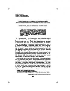
Fig. 1. Conformal parameterization results on high genus surface. 1) Conformal parameterization of genus 16 surface. (2) Conformal parameterization of genus 3 surface. (3) Conformal parameterization computed by double covering. (4) Conformal parameterization of genus 7 surface.

5. Computing Holomorphic 1-form Basis. For each harmonic 1-form, there exists a conjugate harmonic 1-form as defined in Equation22. The problem is to determine the uniqueness of the conjugate harmonic 1-form and find a way to compute it out. Suppose {ω1 , ω2 , · · · , ω2g } is a harmonic 1-form basis. By definition, the conjugate harmonic 1-form ω ∗ should satisfy the following condition (1)

< ωi ∧ ω ∗ , M >=< ωi ∧∗ ω, M >, ∀ωi ∈ H.

130


Because ω ∗ is also harmonic, we can represent it as a linear combination of ωi ’s ω∗ =

(2)

2g X

λk ω k ,

k=1

and we get the following linear system (3)

2g X j=1

λj < ωi ∧ ωj , M >=< ωi ∧∗ ω, M > .

We want to show the linear system 3 is of full rank. We can prove the following theorem: Theorem 5.1. For any harmonic 1-form, its conjugate harmonic 1-form exists and is unique. The proof is not elementary, we will use the duality between homology and cohomology from algebraic topology. Suppose the homology basis are {γ 1 , γ2 , · · · , γ2g }, and (4)

< ωi , γj >= −γi · γj ,

then (5)

< ωi ∧ ωj , M >= γi · γj ,

where · represents the algebraic intersection number between two closed loops. Hence, the linear system in equation 3 is the intersection matrix of homology basis, which is definitely non-degenerated. The solution to Equation 3 exists and is unique. Figure 4.3.1 shows the computation results for several surfaces with high genus numbers. The David sculpture model is with more than ten genus, and the resulting conformal structure is quite accurate. 6. Surfaces With Boundaries. In this section, we want to generalize the method for closed meshes to meshes with boundaries. Given a surface M with boundary ∂M , ∂M 6= φ, we want to compute the global conformal structure for M . We need to compute the holomorphic 1-form on M first. 6.1. Doubling. Given a surface M with boundaries ∂M , we can construct a ˜ , such that M ˜ covers M twice. That is, there exists an symmetric closed surface M ˜ ˜ isometrically to a face isometric projection π : M → M , which maps a face f˜ ∈ M ˜ We call M ˜ a doubling f ∈ M . For each face f ∈ M , there are two preimages in M. of M . The following is the algorithm to compute the doubling of mesh with boundaries. Algorithm 3. Compute Doubling of an Open Mesh Input

: A mesh M with boundary

PERIOD MATRICES

131

˜ Output : The doubling of M , M 1. Make a copy of M , denoted as −M . 2. Reverse the orientation of −M . 3. For any boundary vertex u ∈ ∂ M ,there exists a unique corresponding boundary vertex −u ∈ ∂−M , hence for any edge on e ∈ ∂ M , there exists a unique boundary edge −e ∈ ∂ −M . Find all the correspondences. 4. Glue M and −M , make their corresponding boundary vertices and edges identical. The resulting mesh is ˜. the doubling M

The doubling algorithm is very general for arbitrary surfaces with boundaries, and can be generalized to higher dimensional complexes. The purpose for doubling is to convert the surfaces with boundaries to closed symmetric surfaces. Given a mesh M with boundaries, we would like to compute the basis of holo˜ for M . For each interior morphic 1-forms on M . We first compute the doubling M ˜ , we denote them as u1 and u2 , and say vertex u ∈ M , there are two copies of u in M they are dual to each other, denoted as (1)

u ¯ 1 = u2 , u ¯ 2 = u1 .

˜ , we say u is dual to For each boundary vertex u ∈ ∂M , there is only one copy in M itself, i.e. u ¯ = u. ˜ According to Riemann surface We now compute the harmonic 1-forms on M. ˜ theories [3], all symmetric harmonic 1-forms of M (2)

ω([u, v]) = ω([¯ u, v¯]).

are also harmonic 1-forms on M . Define the dual operator for each harmonic 1-form ω as follows: (3)

ω ¯ ([u, v]) = ω([¯ u, v¯]).

Any ω can be decomposed to a symmetric part and an asymmetric part (4)

ω=

1 1 (ω + ω ¯ ) + (ω − ω ¯ ), 2 2

¯ ) is the symmetric part. where 21 (ω + ω The following algorithm computes the holomorphic 1-form basis for surfaces with boundaries. Algorithm 4. Computing a set of holomorphic 1-form

132


(1) a0

(2) a1

(3) a2

(4) b0

(5) b1

(6) b2

Fig. 1. The homology basis for the genus three sculpture model.

basis for meshes with boundaries. Input : Mesh M with boundaries Output: Holomorphic 1-form basis for mesh M √ √ √ {τ1 + −1τ1∗ , τ2 + −1τ2∗ , · · · , τk + −1τk∗ }. ¯. 1. Compute the doubling of M , M ¯ 2. Compute the harmonic 1-form basis of M {ω1 , ω2 , · · · , ω2g }. 3. Assign τi = 12 (ω + ω ¯ ), remove redundant ones. 4. Compute conjugate harmonic 1-forms of τi , denoted as τ ∗ . 5. Output holomorphic basis √ √ √ {τ1 + −1τ1∗ , τ2 + −1τ2∗ , · · · , τk + −1τk∗ }.

Then, we can use holomorphic 1-form to compute period matrices of M as described in previous section. 7. Experimental Results. We tested our algorithms using real surfaces laser scanned from sculptures and human faces. The surfaces are represented using triangle meshes. The optimization is based on conjugate gradient method, the data structure is mainly half edge boundary representation.

133

PERIOD MATRICES

7.1. Genus Three Sculpture Model. The sculpture model is shown in figure 1 with genus three. The canonical homology basis are also illustrated. The period matrix is computed and display as the following:   0.0143 + 0.6991i -0.0018 + 0.0068i -0.0000 + 0.0067i   (1) R =  -0.0018 + 0.0064i -0.0103 + 1.6003i -0.0047 - 0.1894i  . -0.0000 + 0.0067i -0.0047 - 0.1898i 0.0010 + 1.2844i It is easy to verify that the matrix is symmetric , the imaginary part is positive definite. 7.2. Human Face Surfaces With Feature Regions Removed. The face models are obtained by laser scanning real human faces. We locate the feature curves of the surfaces, and slice the surfaces along these feature curves. We double the result surfaces, and compute the period matrices of them.

(1) female face

(2) male face

(3) female face

(4) male face

Fig. 2. The human face surfaces are preprocessed. In (1) and (2), feature curves are located and the surfaces are sliced along these curves. In (3) and (4), feature points are computed first, then these feature points are removed. The surfaces can be identified by comparing the period matrices.

Figure 7.2 (1) and (2) demonstrate the surfaces with feature regions removed. Figure 7.2 shows the holomorphic one form basis for the female face surface using texturemapping a checkerboard. Figure 7.2 shows the holomorphic one form basis for the male face surface.

(1) ω1

(2) ω2 Fig. 3. Holomorphic one forms on female face model.

(3) ω3

134


(1) ω1

(2) ω1

(3) ω3

Fig. 4. Holomorphic one forms on male face model.

The doubling surfaces are symmetric, the real part of the period matrices are zero. In the following, only the imaginary parts are illustrated. The male surface 7.2 (2) has the following period matrix:   0.6814 0.1642 0.1756 √   (2) −1  0.1642 0.4741 0.1582  , 0.1756 0.1582 0.6474

(3)

The eigen vectors are 

-0.6634   -0.4321 -0.6109

-0.6915 0.0419 0.7212

 0.2860  -0.9009  , 0.3265

0 0.4833 0

 0  0 . 0.3647

The eigen values are 

0.9500  0  0

(4)

The period matrix for the female surface 7.2  0.5335 0.1747 √  −1  0.1747 0.6464 (5) 0.1775 0.1925

(6)


0.4861   0.6121 0.6237

The eigen values are

0.8739 -0.3448 -0.3428

(1) is  0.1775  0.1925  , 0.6540

 -0.0052  -0.7117  , 0.7025

135

PERIOD MATRICES



0.9812  0  0

(7)

0 0.3950 0

 0  0 . 0.4577

7.3. Human Face Surfaces With Feature Points Removed. We locate the feature points on the male face and the female face manually, and punch small holes centered at the feature points as shown in figure 7.2(3) and (4). Then we compute the doubling the surfaces. Because the surfaces are symmetric, the real part of the period matrices are zero. In the following we display the imaginary part. The period matrix of the male surface in 7.2 (3) is  (8)

          

0.9406 0.0821 0.3773 0.1518 0.1719 0.0859 0.2036

0.0821 0.9386 0.1551 0.3824 0.0860 0.1738 0.2096

0.3773 0.1551 1.1511 0.2953 0.2183 0.1488 0.3798

0.1518 0.3824 0.2953 1.1706 0.1477 0.2207 0.3873

0.1719 0.0860 0.2183 0.1477 0.9518 0.1654 0.2781

0.0859 0.1738 0.1488 0.2207 0.1654 0.9557 0.2855

0.2036 0.2096 0.3798 0.3873 0.2781 0.2855 1.3235

           

The eigen vectors for the period matrix are  (9)

          

-0.2830 -0.2889 -0.4401 -0.4495 -0.2800 -0.2848 -0.5303

-0.4842 0.4640 -0.4742 0.4754 -0.2319 0.2136 0.0040

0.3167 0.3150 0.3437 0.3566 -0.3483 -0.3648 -0.5483

-0.5459 0.4781 0.5116 -0.4501 0.0698 -0.0624 -0.0155

0.4957 0.5758 -0.3892 -0.4372 -0.0961 -0.1269 0.2342

0.1635 0.1829 -0.0946 -0.0826 0.5278 0.5316 -0.6024

0 0 0 0 0.6467 0 0

0 0 0 0 0 0.8217 0

0.1214 -0.0919 0.2028 -0.2103 -0.6737 0.6615 -0.0045



     .     

The eigen values for the period matrix are  (10)

          

2.4899 0 0 0 0 0 0

0 1.1251 0 0 0 0 0

0 0 0.9622 0 0 0 0

0 0 0 0.6338 0 0 0

0 0 0 0 0 0 0.7524



     .     

136


The period matrix for the female face surface shown in 7.2 (4) is  (11)

          

1.3530 0.2170 0.2821 0.3944 0.2956 0.3804 0.2053

0.2170 0.9282 0.0921 0.3711 0.1754 0.1617 0.0867

0.2821 0.0921 0.9641 0.1515 0.2020 0.1964 0.1464

0.3944 0.3711 0.1515 1.1036 0.2145 0.3190 0.1637

0.2956 0.1754 0.2020 0.2145 1.0087 0.1539 0.0897

0.3804 0.1617 0.1964 0.3190 0.1539 1.1237 0.3767

0.2053 0.0867 0.1464 0.1637 0.0897 0.3767 0.9245

           

The eigen vectors are  (12)

          

0.5418 0.2868 0.2803 0.4359 0.3022 0.4327 0.2775

0.1011 0.4014 -0.0654 0.3087 0.3468 -0.5458 -0.5576

-0.3935 0.4411 -0.4871 0.4704 -0.3613 0.2067 0.1366

-0.7038 0.1789 0.3904 -0.0350 0.5196 0.0427 0.2175

0.0688 -0.1561 -0.7230 -0.1747 0.6158 0.1553 0.1192

0 0 0 0.8562 0 0 0

0 0 0 0 0.7553 0 0

-0.2015 -0.4985 0.0647 0.3964 0.0817 0.4557 -0.5790

-0.0272 -0.5071 -0.0203 0.5518 0.0446 -0.4883 0.4436



     .     

The eigen values are  (13)

          

2.5050 0 0 0 0 0 0

0 1.0645 0 0 0 0 0

0 0 0.9877 0 0 0 0

0 0 0 0 0 0.6330 0

0 0 0 0 0 0 0.6041



     .     

7.4. Human Face Surfaces With Varying Boundary Conditions.. To test the robustness of our algorithm, we test our algorithm under varying boundary conditions. We cut open three holes in male faces and females faces. The boundary of the faces is cut by a sphere centered at the nose tip point. In practice, the nose tip cannot be located precisely each time. Hence we get different boundary conditions. Figure 7.4 shows the faces with different boundary conditions. We compute and compare the period matrix values under varying boundary conditions. The male surface 7.4(1) has the following period matrix:

(14)



0.7000 √  −1  0.1305 0.1155

0.1305 0.6074 0.1288

 0.1155  0.1288  . 0.6824

137

PERIOD MATRICES

(1)

(2)

(3)

Fig. 5. Human faces under different boundary conditions.

(15)


-0.6246   -0.5108 -0.5907

-0.7078 0.0507 0.7046

 0.3300  -0.8582  . 0.3932

0 0.5757 0

 0  0 . 0.4982


0.9160   0 0

(16)

The male surface 7.4(2) has the following period matrix:   0.7136 0.1362 0.1140 √   (17) −1  0.1362 0.6129 0.1253  . 0.1140 0.1253 0.6637

(18)


-0.6543   -0.5190 -0.5501

-0.6901 0.1122 0.7150

 0.3093  -0.8474  . 0.4315

0 0.5733 0

 0  0 . 0.4994


(19)



0.9175   0 0

The female surface 7.4(3) has the following period matrix:

(20)



0.6221 √  −1  0.1261 0.1384

0.1261 0.7045 0.1355

 0.1384  0.1355  . 0.6722

(4)

138

(21)



0.5117   0.6247 0.5899

0.8114 -0.1257 -0.5708

 0.2824  -0.7707  . 0.5712

0 0.5052 0

 0  0 . 0.5579


0.9357   0 0

(22)

The female surface 7.4(4) has the following  0.6297 0.1244 √  (23) 1  0.1244 0.6868 0.1342 0.1255

(24)


0.5393   0.6125 0.5779

period matrix:  0.1342  0.1255  . 0.6566

0.7875 -0.1236 -0.6038

 0.2984  -0.7808  . 0.5490

0 0.5073 0

 0  0 . 0.5510


(25)



0.9148   0 0

It is to identify these two surfaces by comparing the eigen values of their period matrices. The computation is global, insensitive to the local noise and stable. 8. Summary and Conclusion. This paper introduces algorithms to compute period matrices for real surfaces. The algorithms compute the homology, cohomology, harmonic one form basis and holomorphic one form basis. The algorithms are intrinsic to the geometry of the surfaces, independent of the data construction, insensible to the noise. By Riemann uniformization theory, all compact surfaces can be conformally mapped to sphere, disk, or plane. We can find a triangulation with all sharp angles for these canonical spaces and map the triangulations to the surface. If the triangulation is dense enough, then the triangulation on the surfaces are with all acute angles. Period matrices can be used for surface classification, surface recognition. It is a challenging problem to qualitatively measure the dependency between the period matrices and the Riemann metric tensor. We will do future research along this direction and find more applications for period matrices.

PERIOD MATRICES

139

REFERENCES [1] P. Alliez, M. Meyer, and M. Desbrun. Interactive geomety remeshing. In SIGGRAPH 02, pages 347–354, 2002. [2] S Angenent, S Haker, A Tannenaum, and R Kikinis. Conformal geometry and brain flattening. MICCAI, pages 271–278, 1999. [3] E. Arbarello, M. Cornalba, P. Griffiths, and J. Harris. Topics in the Theory of Algebraic Curves. 1938. [4] T. Duchamp, A. Certian, A. Derose, and W. Stuetzle. Hierarchical computation of pl harmonic embeddings. preprint, 1997. [5] X. Gu, Y. Wang, T. Chan, P.M. Thompson, and S.-T. Yau. Brain surface conformal mapping. In Human Brain Mapping, 2003. [6] X. Gu, Y. Wang, T. Chan, P.M. Thompson, and S.-T. Yau. Genus zero surface conformal mapping and its application to brain surface mapping. In Information Processing in Medical Imaging, 2003. [7] X. Gu and S.-T Yau. Global conformal surface parameterization. In ACM Symposium on Geometry Processing, pages 127–137, 2003. [8] X. Gu and S.-T Yau. Surface classification using conformal structures. In International Conference on Computer Vision, 2003. [9] X. Gu and S.T. Yau. Computing conformal structures of surafces. Communication of Informtion and Systems, December 2002. [10] S. Haker, S. Angenent, A. Tannenbaum, R. Kikinis, G. Sapiro, and M.Halle. Conformal surface parameterization for texture mapping. IEEE Transactions on Visualization and Computer Graphics, 6:240–251, April-June 2000. [11] I. Kra and H. M. Farkas. Riemann Surfaces. Springer-Verlag New York, Incorporated, 1995. [12] B. Levy and J.L. Mallet. Non-distorted texture mapping for sheared triangulated meshes. In SIGGRAPH 98, pages 343–352. [13] B. Levy, S. Petitjean, N. Ray, and J. Maillot. Least squares conformal maps for automatic texture atlas generation. In SIGGRAPH 02, pages 362–371, 2002. [14] Y. Wang, X. Gu, T. Chan, P.M. Thompson, and S.-T. Yau. Intrinsic brain surface conformal mapping using a variational method. In SPIE International Symposium on Medical Imaging, 2004.