Computing Contour Closure. James H. Elder1 and Steven W. Zucker2. 1 NEC Research Institute, Princeton, NJ, U.S.A.. 2 Centre for Intelligent Machines, McGill ...
Computing Contour Closure James H. Elder1 and Steven W. Zucker2 2
1
NEC Research Institute, Princeton, NJ, U.S.A. Centre for Intelligent Machines, McGill University, Montr�eal, Canada.
Abstract. Existing methods for grouping edges on the basis of local
smoothness measures fail to compute complete contours in natural images: it appears that a stronger global constraint is required. Motivated by growing evidence that the human visual system exploits contour closure for the purposes of perceptual grouping [6, 7, 14, 15, 25], we present an algorithm for computing highly closed bounding contours from images. Unlike previous algorithms [11, 18, 26], no restrictions are placed on the type of structure bounded or its shape. Contours are represented locally by tangent vectors, augmented by image intensity estimates. A Bayesian model is developed for the likelihood that two tangent vectors form contiguous components of the same contour. Based on this model, a sparsely-connected graph is constructed, and the problem of computing closed contours is posed as the computation of shortest-path cycles in this graph. We show that simple tangent cycles can be e�ciently computed in natural images containing many local ambiguities, and that these cycles generally correspond to bounding contours in the image. These closure computations can potentially complement region-grouping methods by extending the class of structures segmented to include heterogeneous structures.
1 Introduction We address the problem of computing closed bounding contours in real images. The problem is of interest for a number of reasons. A basic task of early vision is to group together parts of an image that project from the same structure in a scene. Studies of perceptual organization have demonstrated that the human visual system exploits a range of regularities in image structure to solve this task [12, 14, 28]. Inspired in part by these studies, algorithms have been developed to apply continuity, cocircularity and smoothness constraints to organize local edges into extended contours [2,10,17,19,22,24]. However, despite persuasive psychophysical demonstrations of the role of contour closure in perceptual organization [6, 7, 14, 15, 25], closure constraints for computer vision algorithms have been largely ignored (although see [1, 11]). This is surprising, since existing algorithms, while capable of producing extended chains of edges, are seldom successful in grouping complete contours. Closure is a potentially powerful cue that could complement smoothness cues to allow more complete contours to be computed. In natural images, contours are fragmented due to occlusions and other effects, making local grouping cues weak and unreliable. While these local cues
may be summed or otherwise integrated along a contour to form global measures of \smoothness", \likelihood" or \salience", such a global measure is as weak as its weakest local constituent. This is illustrated in Fig. 1(a): the most plausible continuation of a contour viewed locally may be clearly incorrect when viewed in global context. This error is not revealed in a summation of local grouping cues over the curve, since both the correct and the incorrect continuations lead to similar measures. A global feature is needed which is far more sensitive to such local errors. Closure is a potentially powerful feature because a single local error will almost certainly lead to a low measure of closure.
a
% Correct
100
b a
90 80 70
b 60 50
0
5
10
15
20
Binding contrast (%)
(a)
(b)
(c)
Fig. 1. (a) Locally, the most plausible continuation of fragment a is through frag-
ment b. Given global context, fragments instead group to form simple cycles with high measures of closure. (b) A region grouping algorithm would segment this image into 12 disjoint regions, yet human observers see two overlapping objects. Regularities of the object boundaries must be exploited. (c) Psychophysical data for shape identi cation task. Subjects must discriminate between a fragmented concave shape (shown) and a 1-D equivalent convex shape (not shown), at very low contrasts. Results show that contour closure cues greatly enhance performance. No e�ect of texture cues is observed. From [8]. The computation of closed contours is also potentially useful for grouping together image regions which project from common structures in the scene: objects, parts of objects, shadows and specularities. Existing techniques for region grouping apply homogeneity or smoothness constraints on luminance, colour or texture measures over regions of the image (e.g. 16, 20, 21). These techniques have inherent limitations. While a region-grouping algorithm would segment the image of Fig. 1(b) into 12 disjoint components, human observers perceive two irregularly painted, overlapping objects. Since these are nonsense objects, our inference cannot be based on familiarity. We must be using the geometry of the boundaries to group the objects despite their heterogeneity. This situation is not arti cial. Objects are often highly irregular in their sur-
face re ectance functions, and may be dappled in irregular ways by shadows and specularities. While surface markings, shadows and specularities fragment image regions into multiple components, geometric regularities of bounding contour persist. Contour closure is thus potentially important for segmentation because it broadens the class of structures that may be segmented to include such heterogeneous structures. Interestingly, recent psychophysical experiments [8] suggest that contour grouping cues such as closure may be more important than regional texture cues for the perceptual organization of 2-D form (Fig. 1(c)).
2 Previous Work The problem of contour grouping has been approached in many di�erent ways. Multi-scale smoothness criteria have been used to impose an organization on image curves [4,17,22], sequential methods for tracking contours within a Bayesian framework have recently been developed [2] and parallel methods for computing local \saliency" measures based on contour smoothness and total arclength have been studied [1, 24]. In general, these techniques are capable of grouping edge points into extended chains. However, no attempt is made to compute closed chains; a necessary condition for computing global 2-D shape properties and for segmenting structures from an image. A separate branch of research investigates the grouping of occlusion edges into complete contours, ordered in depth [18,26]. While interesting from a theoretical point of view, a large fraction of the edges in real images are not occlusion edges, and a recent study [5] suggests that it is not possible to locally distinguish occlusion edges from other types of edges. It is our view that algorithms for grouping contours must work for all types of structure in an image (e.g. objects, shadows, surface markings). Jacobs [11] has studied the problem of inferring highly-closed convex cycles of line segments from an image, to be used as input for a part-based object recognition strategy. Given the generality of boundary shape, it is clearly of great interest to determine whether bounding contours can be recovered without such restrictive shape constraints. Most similar to our work is a very recent study by Alter [1] on the application of shortest-path algorithms to the computation of closed image contours. While similar in concept, these two independent studies di�er substantially in their implementation.
3 Overview of the Algorithm Our goal here is to recover cycles of edge points which bound two-dimensional structures in an image. The algorithm is to be fully automatic and no restrictions are placed on the type of structure bounded or its shape. Since no constraint of disjointness is imposed, in principle the bounding contours of an entire object, its parts, markings, and shadows can be recovered. Image contours are represented locally as a set of tangent vectors, augmented by image intensity estimates. A Bayesian model is developed to estimate the
likelihoods that tangent pairs form contiguous components of the same image contour. Applying this model to each tangent in turn allows the possible continuant tangents for each tangent to be sorted in order of their likelihood. By selecting for each tangent the 6 most likely continuant tangents, a sparse (6connected), weighted graph is constructed, where the weights are the computed pairwise likelihoods. By assuming independence between tangent pair likelihoods, we show that determining the most probable tangent cycle passing through each tangent can be posed as a shortest path computation over this sparse graph. We can therefore use standard algorithms (e.g. Dijkstra's algorithm [23]) to solve this problem in low-order polynomial time.
4 Extended Tangents Edges are detected by a multi-scale method which automatically adapts estimation scale to the local signal strength and provides reliable estimates of edge position and tangent orientation [9]. In addition to the geometric properties of position and orientation, we make use of local image intensity estimates provided by our edge detector. Due to uncertainty induced by discretization and sensor noise, contours generate noisy, laterally-displaced local edges (Fig. 2(a)). Tracing a contour through these local tangents generates a curve corrupted by wiggles due to sensing artifacts. Also, due to blurring of the luminance function at the imaging and estimation stages, edge estimates near corners and junctions are corrupted (Fig. 2(b)).
? ?
(a)
(b)
Fig. 2. (a) The set of raw tangent estimates for a contour. Imposing an order-
ing on these local tangent estimates generates a contour distorted by sampling artifacts. (b) The smoothing of the image at the sensing and estimation stages corrupts tangent estimates near contour junctions and corners. Achieving a more reliable local representation requires more global constraints. Here, we introduce a method for re ning local edge information based on an extended tangent representation, which represents a curve as a sequence
of disjoint line segments. Each local edge in the image generates a tangent line passing through the edge pixel in the estimated tangent direction. The subset of tangent estimates which are 8-connected to the local edge and which lie within an �-neighbourhood of the local tangent line are identi ed with the extended tangent model. The algorithm for selecting extended tangents to approximate a contour is illustrated in Fig. 3. Given a connected set of local edges, the longest line segment which faithfully models a subset of these is determined. This subset is then subtracted from the original set. This process is repeated for the connected subsets thus created until all local edges have been modeled.
(a)
(b)
(c)
Fig. 3. Computing the extended tangent representation. (a) For each connected
set of edge pixels, the subset of pixels underlying the longest extended tangent is selected. (b) The edge points thus modeled are subtracted. (c) The process is repeated for each connected set of edge pixels thus spawned. Since the extended tangents selected must be consistent with the global geometry of the curves, they provide more accurate estimates of contrast and tangent orientation than do the corrupted local edges near the junction. The extended tangent algorithm is conceptually simpler than most methods for computing polygonal approximations [20], and does not require preprocessing of the edge map to link local edges into ordered lists, as is required for most other methods (e.g. 11,17,20).
5 A Bayesian Model for Tangent Grouping The extended tangent representation leads naturally to a representation for global contours as tangent sequences: De nition 1. A tangent sequence t1 ! ::: ! tn is an injective mapping from a nite set of integers to a set of extended tangents. The injective property restricts our de nition to sequences which do not pass through the same extended tangent twice. The identi cation of extended
tangents with integers imposes an ordering on the tangents which distinguishes a tangent sequence from an arbitrary clutter of tangents. If a contour bounds a 2-D structure in the image, this sequence will come back on itself. Thus bounding contours are represented as cycles of extended tangents, t1 ! ::: ! tn ! t1 ! ::: By this de nition, any ordered set of tangents in an image can form a tangent sequence. In order to compute bounding contours, some measure of the likelihood of a tangent sequence must be established. For this purpose, we develop a Bayesian model for estimating the posterior probability of a tangent sequence given data on the geometric and photometric relations between adjacent tangent tuples of the sequence. We will begin by assuming that tangent links are independent: i.e.
p(t1 ! ::: ! tn ) = p(t1 ! t2 )p(t2 ! t3 ):::p(tn,1 ! tn ) This approximation will greatly simplify the computation of tangent sequence likelihoods, reducing likelihood estimation for a tangent sequence to the problem of estimating the likelihoods of its constituent links. The likelihood that two tangents project from the same contour is modeled as the probability of their rectilinear completion (Fig. 4), so that the probability of a link depends on the following observables (see Sections 6 and 7 for details of the model): 1. 2. 3. 4.
The lengths l1 and l2 of the extended tangents. The length r of the straight-line interpolant. The 2 orientation changes �a and �b induced by the interpolation. The di�erences in estimated image intensity �ih , �il on the bright side and the dark side of the tangents, respectively.
i l1 t1
l ih11
i l2
θb
θa
r
l2
t h2 2
i
Fig. 4. Rectilinear interpolation model.
Setting o = fl1; l2 ; r; �a ; �b ; �ih; �il g, Bayes' theorem can be used to express the posterior probability of a link from tangent t1 to t2 (called the \link hypothesis") in terms of the likelihoods of the observables:
p(t1 ! t2 jo) = p(ojt1 ! pt2()op)(t1 ! t2 )
Letting t1 ! = t2 represent the hypothesis that t2 is not the continuant of t1 (the \no-link hypothesis"), the evidence p(o) can be expanded as p(o) = p(ojt1 ! t2 )p(t1 ! t2 ) + p(ojt1 != t2 )p(t1 != t2 ): It is convenient to rewrite the posterior probability as p(t1 ! t2 jo) = (1 +1LP ) where p(t1 != t2 ) = t2 ) L = pp((oojjtt1 ! ! t ) P = p(t ! t ) 1
2
1
2
The prior ratio P represents the ratio of the probability that a curve ends at t1 , to the probability that the curve continues. For most images, curves are expected to continue over many tangents. It is therefore appropriate to choose a large value for the prior ratio: in our experiments we use P = 50. The likelihood ratio L represents the ratio of the likelihood of the observables given that t2 is not a continuant of t1 to their likelihood given that t2 is a continuant of t1 . Models for these likelihoods are developed in the next two sections.
6 Link Hypothesis Likelihoods In order to model the link hypothesis likelihoods p(ojt1 ! t2 ) we must consider the distinct events that can split the image curve into two separate extended tangents t1 and t2 . The three possible hypotheses for a tangent split considered are termed respectively the curvature, interruption and corner hypotheses: Curvature The contour is curving smoothly: two tangents are needed to model the local edges to � accuracy. Relatively small values for r, �a and �b are expected. Interruption The contour is interrupted, for example by an occlusion, shadow, or loss of contrast. We expect potentially large values for r, but again relatively small values for �a and �b . Corner The contour corners sharply: two tangents are generated on either side of the corner. We expect a relatively small value for r, but possibly large values for �a and �b . Since each of these hypotheses generates di�erent expectations for the observables, the corresponding link hypothesis likelihoods are decomposed into likelihoods for the 3 disjoint events:
p(ojt1 ! t2 ) = p(ojt1 ! t2 ; curvature)p(curvature) + p(ojt1 ! t2 ; interruption)p(interruption) + p(ojt1 ! t2 ; corner)p(corner)
In a natural world of piecewise-smooth objects, the curvature hypothesis is the most likely. For our experiments we assign
p(curvature) = 0:9 and p(interruption) = p(corner) = 0:05: Combining the observables l1 ; l2 and r into a normalized gap length r0 , r0 = minfrl ; l g 1 2 we write a summarized set of observables as o0 = fr0 ; �a ; �b ; �b; �dg. Approximating these as conditionally independent on the 3 tangent split hypotheses, we use half-Gaussian functions to model the link hypothesis likelihoods for each observables oi :
p , oi 2 p(oi jt1 ! t2 ) = p��2 e 2�o2i ; oi > 0:
oi The scale constants �oi used in this paper are shown in Table 1.
�r �r ��a = ��b ��b = ��d (pixels) (pixels) (deg) (grey levels) curvature 2 10 20 interruption 0.5 10 20 corner 2 90 20 0
Table 1. Scale constants for link hypothesis likelihood functions
7 No-Link Hypothesis Likelihoods Modelling the position of a tangent as a uniform distribution over the image domain, for an L � L image, and r