Computing Finite Models by Reduction to Function-Free Clause Logic Peter Baumgartner National ICT Australia (NICTA)
[email protected] Hans de Nivelle Max-Planck-Institute f¨ur Informatik
[email protected]
Alexander Fuchs Department of Computer Science The University of Iowa
[email protected] Cesare Tinelli Department of Computer Science The University of Iowa
[email protected]
August 19, 2006
Abstract Recent years have seen considerable interest in procedures for computing finite models of first-order logic specifications. One of the major paradigms, MACEstyle model building, is based on reducing model search to a sequence of propositional satisfiability problems and applying (efficient) SAT solvers to them. A problem with this method is that it does not scale well, as the propositional formulas to be considered may become very large. We propose instead to reduce model search to a sequence of satisfiability problems made of function-free first-order clause sets, and to apply (efficient) theorem provers capable of deciding such problems. The main appeal of this method is that first-order clause sets grow more slowly than their propositional counterparts, thus allowing for more space efficient reasoning. In the paper we describe the method in detail and show how it is integrated into one such prover, Darwin, our implementation of the Model Evolution calculus. The results are general, however, as our approach can be used in principle with any system that decides the satisfiability of function-free first-order clause sets. To demonstrate its practical feasibility, we tested our approach on all satisfiable problems from the TPTP library. Our methods can solve a significant subset of these problems, which overlaps but is not included in the subset of problems solvable by state-of-the-art finite model builders such as Paradox and Mace4.
1
2
1
1
Introduction
Introduction
Methods for model computation can be classified as those that directly search for a finite model, like the extended PUHR tableau method [BT98], the methods in [Bez05, dNM06] and the methods in the SEM-family [Sla92, ZZ95, McC03], and those based on transformations into certain fragments of logic and relying on corresponding readily available systems (see [BS06] for a recent approach). The latter approach includes the family of MACE-style model builders [McC03]. These systems search for finite models, essentially, by searching the space of interpretations with domain sizes 1, 2, . . ., in increasing order, until a model is found. The MACE-style model builder with the best performance today is perhaps the Paradox system [CS03]. We present in this paper a new approach in the MACE/Paradox tradition which however capitalizes on new advances in instantiation-based first-order theorem proving, as opposed to advances in propositional satisfiability as in the case of MACE and Paradox. The general idea in our approach is the same: to find a model with n elements for a given a clause set possibly with equality, the clause set is first converted into a simpler form by means of the following transformations. 1. Each clause is flattened. 2. Each n-ary function symbol is replaced by an n + 1-ary predicate symbol and equality is eliminated. 3. Clauses are added to the clause set that impose totality constraints on the new predicate symbols, but over a domain of cardinality n. The details of our transformation differ in various aspects from the MACE/Paradox approach. In particular, we add no functionality constraints over the new predicate symbols. The main difference, however, is that we evenually reduce the original problem to a satisfiability problem over function-free clause logic (without equality), not over propositional logic. As a consequence of the different target logic, we do not use a SAT solver to look for models. Instead, we use a variant of Darwin [BFT06a], our implementation of the Model Evolution calculus [BT03], which can decide satisfiability in that logic. While we do take advantage of some of the distinguishing features of Darwin and the Model Evolution calculus, especially in the way models are constructed, our method is general enough that it could use without much additional effort any other decision procedure for function-free clause logic, for instance, any implementation of one of the several instance-based methods for first-order reasoning that are currently enjoying a growing popularity. In this paper we illustrate our method in some detail, presenting the main translation and its implementation within Darwin, and discussing our initial experimental
3
results in comparison with Paradox itself and with Mace4 [McC03], a competitive, nonMACE-like (despite the name) model builder. The results indicate that our method is rather promising as it can solve 1074 of the 1251 satisfiable problems in the TPTP library [SS98]. These problems are neither a subset nor a superset of the sets of 1083 and 802 problems respectively solved (under the same experimental settings) by Paradox and Mace4.
2
Preliminaries
We use standard terminology from automated reasoning. We assume as given a signature Σ = ΣF ∪ ΣP of function symbols ΣF (including constants) and predicate symbols ΣP . As we are working (also) with equality, we assume ΣP contains a distinguished binary predicate symbol ≈, used in infix form, with 6≈ denoting its negation. Terms, atoms, literals and formulas over Σ and a given (denumerable) set of variables V are defined as usual. A clause is a (finite) implicitly universally quantified disjunction of literals. A clause set is a finite set of clauses. We use the letter C to denote clauses and the letter L to denote literals. For a given atom P(t1 , . . . ,tn ) (possibly an equation) the terms t1 , . . . ,tn are also called the top-level terms (of P(t1 , . . . ,tn )). With regards to semantics, we use the notions of (first-order) satisfiability and Esatisfiability in a completely standard way. If I is an (E-)interpretation then |I| denotes the domain (or universe) of I. Recall that in E-interpretations the equality relation is interpreted as the identity relation, i.e. for every E-interpretation I it holds ≈I = {(d, d) | d ∈ |I|}. We are primarily interested in computing finite models, which are models (of the given clause set) with a finite domain. In the remainder of the paper, we assume that M is a given (finite) clause set over signature Σ = ΣF ∪ ΣP , where ΣF (resp. ΣP ) are the function symbols (resp. predicate symbols) occuring in M.
3
Finite Model Transformation
In this section we give a general description of the tranformations we apply to the input problem to reduce it to an equisatisfiable problem in function-free clause logic without equality. We do that by defining various transformation rules on clauses. In the rules, we write L ∨ C C0 ∨ C to indicate that the clause C0 ∨ C is obtained from the clause L ∨C by (single) application of one of these rules.
4
3
3.1
Finite Model Transformation
Basic Transformation
(1) Abstraction of positive equations. s ≈ y ∨C
s 6≈ x ∨ x ≈ y ∨C
x ≈ t ∨C
t 6≈ y ∨ x ≈ y ∨C
s ≈ t ∨C
s 6≈ x ∨ t 6≈ y ∨ x ≈ y ∨C
if s is not a variable and x is a fresh variable if t is not a variable and y is a fresh variable if s and t are not variables and x and y are fresh variables
These rules make sure that all (positive) equations are between variables. (2) Flattening of non-equations. (¬)P(. . . , s, . . .) ∨C
(¬)P(. . . , x, . . .) ∨ s 6≈ x ∨C
if P 6= ≈, s is not a variable, and x is a fresh variable
(3) Flattening of negative equations. f (. . . , s, . . .) 6≈ t ∨C
f (. . . , x, . . .) 6≈ t ∨ s 6≈ x ∨C
if s is not a variable and x is a fresh variable
(4) Separation of negative equations. s 6≈ t ∨C
s 6≈ x ∨ t 6≈ x ∨C
if neither s nor t is a variable, and x and y are fresh variables
This rule makes sure that at least one side of a (negative) equation is a variable. Notice that this property is also satisfied by the transformations (2) and (3). (5) Removal of trivial negative equations. x 6≈ y ∨C
Cσ where σ = {x 7→ y}
(6) Orientation of negative equations. x 6≈ t ∨C
t 6≈ x ∨C
if t is not a variable
For a clause C, let the basic transformation of C, denoted as B (C), be the clause obtained from C by applying the transformations (1)-(6), in this order, each as long as possible.1 We extend this notation to clause sets in the obvious way, i.e., B (M) is the clause set consisting of the basic transformation of all clauses in M. The two flattening transformations alone, when applied exhaustively, turn a clause into a flat one, where a clause is flat if: 1 It
is easy to see that this process always terminates.
3.2
Conversion to Relational Form
5
1. each top-level term of each of its negative equations is a variable or has the form f (x1 , . . . , xn ), where f is a function symbol, n ≥ 0, and x1 , . . . , xn are variables; 2. each top-level term of each of its non-equations is a variable. Similar flattening transformations have been considered before as a means to deal more efficiently with equality within calculi for first-order logic without equality [Bra75, BGV98]. The basic transformation above is correct in the following sense. Lemma 3.1 (Correctness of B ) The clause set M is E-satisfiable if and only if B (M) is E-satisfiable. Proof. That flattening preserves E-satisfiability (both ways) is well-know (cf. [Bra75]). Regarding transformations (1), (4), (5) and (6), the proof is straightforward or trivial.
3.2
Conversion to Relational Form
It is not hard to see that, for any clause C, the following holds for the clause set B (C): 1. each of its positive equations is between two variables, 2. each of its negative equations is flat and of the form f (x1 , . . . , xn ) 6≈ y, and 3. each of its non-equations is flat. After the basic transformation, we apply the following one, turning each n-ary function symbol f into a (new) n + 1-ary predicate symbol R f . (7) Elimination of function symbols. f (x1 , . . . , xn ) 6≈ y ∨C
¬R f (x1 , . . . , xn , y) ∨C
Let BR (M) be the clause set obtained from an exhaustive application of this transformation to B (M). Recall that an n + 1-ary relation R over a set A is left-total if for every a1 , . . . , an ∈ A there is an b ∈ A such that (a1 , . . . , an , b) ∈ R. The relation R is right-unique if whenever (a1 , . . . , an , b) ∈ R there is no other tuple of the form (a1 , . . . , an , b0 ) in R. Because of the above properties (1)–(3) of B (M), the transformation BR (M) is welldefined, and will produce a clause set with no function symbols. This transformation however is not unsatisfiability preserving unless one considers only left-total interpretations for the predicate symbols R f . More formally:
6
3
Finite Model Transformation
Lemma 3.2 (Correctness of BR ) The clause set M is E-satisfiable if and only if there is an E-model I of BR (M) such that (R f )I is left-total, for every function symbol f ∈ ΣF . Proof. The direction from left to right is easy. For the other direction, let I be an E-model of BR (M) such that (R f )I is left-total for every function symbol f ∈ ΣF . Recall that functions are nothing but left-total and right-unique relations. We will show how to obtain from I an E-model I0 of BR (M), that preserves left-totality and adds 0 right-uniqueness, i.e., such that (R f )I is both left-total and right-unique for all f ∈ ΣF . Since such an interpretation is clearly a model of B (M), it will the follow immediately by Lemma 3.1 that M is E-satisfiable. 0 We obtain I0 as the interpretation that is like I, except that (R f )I contains exactly one element (d1 , . . . , dn , d), for every d1 , . . . , dn ∈ |I|, chosen arbitrarily from (R f )I (this 0 choice exists because (R f )I is left-total). It is clear from the construction that (R f )I is right-unique and left-total. Trivially, I0 interpretes ≈ as the identity relation, because I does, as I is an E-interpretation. Thus, I0 is an E-interpretation, too. It remains to prove that with I being a model of BR (M) then so is I0 . This follows from the fact that every occurrence of a predicate symbol R f , with f ∈ ΣF , in the clause 0 set BR (M) is in a negative literal. But then, since (R f )I ⊆ (R f )I by construction, it follows immediately that any clause of BR (M) satisfied by I is also satisfied by I0 . The significance of this lemma is that it requires us to interpret the predicate symbols R f as left-total relations, but not necessarily as right-unique ones. Consequently, rightuniqueness will not be axiomatized below.
3.3
Addition of Finite Domain Constraints
To force left-totality, one could add the Skolemized version of axioms of the form ∀x1 , . . . , xn ∃y R f (x1 , . . . , xn , y) to Br (M). The resulting set would be E-satisfiable exactly when M is E-satisfiable.2 However, since we are interested in finite satisfiability, we use finite approximations of these axioms. To this end, let d be a positive integer, the domain size. We consider the expansion of the signature of Br (M) by d fresh constant symbols, which we name 1, . . . , d. Intuitively, instead of the totality axiom above we can now use the axiom ∀x1 , . . . , xn ∃y ∈ {1, . . . , d} R f (x1 , . . . , xn , y) . Concretely, if f is an n-ary function symbol let the clause R f (x1 , . . . , xn , 1) ∨ · · · ∨ R f (x1 , . . . , xn , d) 2 Altogether,
this proves the (well-known) result that function symbols are “syntactic sugar”. They can always be eliminated in an equisatisfiability preserving way, at the cost of introducing existential quantifiers.
3.4
Symmetry Breaking
Rc1 (1) ∨ · · · ∨ Rc1 (d) Rc2 (1) ∨ · · · ∨ Rc2 (d)
7
Rc1 (1) Rc2 (1) ∨ Rc2 (2) .. . Rcd (1) ∨ · · · ∨ Rcd (d) Rcd+1 (1) ∨ · · · ∨ Rcd+1 (d) .. .
.. .
Rcm (1) ∨ · · · ∨ Rcm (d) (a)
Rcm (1) ∨ · · · ∨ Rcm (d) (b)
Figure 1: Totality axioms for constants and their triangular form be the d-totality axiom for f , and let D (d) be the set of all d-totality axioms for all function symbols f ∈ ΣF . The set D (d) axiomatizes the left-totality of (R f )I , for every function symbol f ∈ ΣF and interpretation I with |I| = {1, . . . , d}.
3.4
Symmetry Breaking
Symmetries have been identified as a major source for inefficiencies in constrain solving systems. Value symmetry applies to a problem when a permutation of the values (or better, value vector) assigned to variables constitutes a solution to the problem, too. A dual symmetry property may apply to the (decision) variables of a problem, giving rise to variable symmetry. Breaking such symmetries has been recognized as a source for considerable efficiency gains. It is easy to break some value symmetries introduced by assigning domain values to constants. Suppose ΣF contains m constants c1 , . . . , cm . Recall that D (d) contains, in particular, the axioms shown in Figure 1(a). Similarly to what is done with Paradox, these axioms can be replaced by the more “triangular” form shown in Figure 1(b). This form reflects symmetry breaking of assigning values for the first d constants. In fact, one could further strengthen the symmetry breaking axioms by adding (unit) clauses like ¬Rc1 (2), . . . ¬Rc1 (d). We do not add them, as they do not constrain the search for a model further (they are all pure). In the sequel we will refer to the clause set as described here as D (d).
3.5
Putting all Together
Since we want to use clause logic without equality as the target logic of our overall transformation, the only remaining step is the explicit axiomatization of the equality symbol ≈ over domains of size d—so that we can exploit Lemma 3.2 in the (interesting)
8
4
Implementation
right-to-left direction. This is easily achieved with the clause set
E (d) = {i 6≈ j | 1 ≤ i, j ≤ d and i 6= j} . Finally then, we define the finite-domain transformation of M as the clause set
F (M, d) := BR (M) ∪ D (d) ∪ E (d) . Putting all together we arrive at the following first main result: Theorem 3.3 (Correctness of the Finite-Domain Translation) Let d be a positive integer. Then, M is E-satisfiable by some finite interpretation with domain size d if and only if F (M, d) is satisfiable. Proof. Follows from Lemma 3.2 and the comments above on D (d) and E (d), together with the observation that if F (M, d) is satisfiable it is satisfiable in a Herbrand interpretation with universe {1, . . . , d}. More precisely, for the only-if direction assume as given a Herbrand model I of F (M, d) with universe {1, . . . , d}. It is clear from the axioms E (d) that I assigns false to the equation (d 0 ≈ d 00 ), for any two different elements d 0 , d 00 ∈ {1, . . . , d}. Now, the model I can be modified to assign true to all equations d 0 ≈ d 0 , for all d 0 ∈ {1, . . . , d} and the resulting E-interpretation will still be a model for F (M, d). This is, because the only occurences of negative equations in F (M, d) are those contributed by E (d), which are still satisfied after the change.3 It is this modified model that can be turned into an E-model of M. This theorem suggests immediately a (practical) procedure to search for finite models, by testing F (M, d) for satisfiability, with d = 1, 2, . . ., and stopping as soon as the first satisfiable set has been found. Moreover, any reasonable such procedure will return in the satisfiable case a Herbrand representation (of some finite model). Indeed, the idea of searching for a finite model by testing satisfiability over finite domains of size 1, 2, . . . is implemented in our approach and many others (Paradox [CS03], Finder [Sla92], Mace [McC94], Mace4 [McC03] , SEM [ZZ95] to name a few).
4
Implementation
We implemented the transformation described so far within our theorem prover Darwin. In addition to being a full-blown theorem prover for first-order logic without equality, Darwin is a decision procedure for the satisfiability of function-free clause sets, and thus is a suitable back-end for our transformation. We call the combined system FM-Darwin (for Finite Models Darwin). 3 Notice,
in particular, that BR (M) contains only positive occurences of equations, if any.
9
Conceptually, FM-Darwin builds on Darwin by adding to it as a front-end an implementation of the transformation F (Section 3.5), and invoking Darwin on F (M, d), for d = 1, 2, ..., until a model is found. In reality, FM-Darwin is built within Darwin and differs from the conceptual procedure described so far in the following ways: 1. The search for models of increasing size is built in Darwin’s own restarting mechanism. For refutational completeness Darwin explores its search space in an iterativedeepening fashion with respect of certain depth measures. The same mechanism is used in FM-Darwin to restart the search with an increased domain size d + 1 if the input problem has no models of size d. 2. FM-Darwin implements some obvious optimizations over the transformation rules described in Section 3. For instance, the tranformations (1)–(4) are done in parallel, depending on the structure of the current literal. Transformation (6) is done implicitly as part of tranformation (7), when turning equations into relations. Also, when flattening a clause, the same variable is used to abstract different occurrences of a subterm. 3. Because the clause sets F (M, d) and F (M, d + 1), for any d, differ only in the their subsets D (d) ∪ E (d) and D (d + 1) ∪ E (d + 1), respectively, there is no need to regenerate the constant part, and this is not done. 4. Similarly to SAT solvers based on the DPLL procedure, Darwin has the ability to learn new (entailed) clauses—or lemmas—in failed branches of a derivation, which is helpful to prune search space in later branches [BFT06b]. Some of the learned lemmas are independent from the current domain size and so can be carried over to later iterations with larger domain sizes. To do that, each clause in D (d + 1) is actually guarded by an additional literal Md standing for the current domain size. In FM-Darwin, lemmas depending on the current domain size d, and only those, retain the guard Md when they are built, making it easy to eliminate them when moving to the next size d + 1. 5. Recall from step (7) in the transformation (Section 3.2) that every function symbol is turned into a predicate symbol. In our actual implementation, we go one step further and use a meta modeling approach that can make the final clause set produced by our translation more compact, and possibly speed up the search as well, thanks to the way models are built in the Model Evolution calculus. The idea is the following. For every n > 0, instead of generating an n + 1-ary relation symbol R f for each n-ary function symbol f ∈ ΣF we use an n + 2-ary relation symbol Rn , for all n-ary function symbols. Then, instead of translating a literal of the form f (x1 , ..., xn ) 6≈ y into the literal ¬R f (x1 , ..., xn , y), we translate it into the literal Rn ( f , x1 , ..., xn , y), treating f as a zeroarity symbol. The advantage of this translation is that instead of needing one totality axiom per relation symbol R f with f ∈ ΣF we only need one per function symbol arity
10
4
(among those found in ΣF ).
4
Implementation
The d-totality axioms then take the more general form
Rn (y, x1 , . . . , xn , 1) ∨ · · · ∨ Rn (y, x1 , . . . , xn , d) where the variable y is meant to be quantified over the (original) function symbols in ΣF . Note that the zero-arity symbols representing the original function symbols in the input are in addition to the domain constants, and of course never interact with them.5 6. Like Paradox, FM-Darwin performs a kind of sort inference in order to improve the effectiveness of symmetry breaking. Each function and predicate symbol of arity n in Σ is assigned a type respectively of the form S1 × . . . × Sn → Sn+1 and S1 × . . . × Sn , where all sorts Si are initially distinct. Each term in the input clause set is assigned the result sort of its top symbol. Two sorts Si and S j are then identified based on the input clause set by applying a union-find algorithm with the following rules. First, all sorts of different occurrences of the same variable in a clause are identified; second, the result sorts of two terms s and t in an equality s ≈ t are identified; third, for each term or atom of the form f (. . . ,t, . . .) the argument sort of f at t’s position is identified with the sort of t. All sorts left at the end are assumed to have the same size. This way, when a sorted model is found (with all sorts having some size d), it can be translated into an unsorted model by an isomorphic translation of each sort into a single domain of size d. This implies that one can conceptually search for a sorted model and apply the symmetry breaking rules independently for each sort, and otherwise do everything else as described in the previous section. In addition to generally improving performance, this makes the whole procedure less fragile, as the order in which the constants are chosen for the symmetry breaking rules can have a dramatic impact on the search space. 7. Splitting clauses. Paradox and Mace2 use transformations that, by introducing new predicate symbols, can split a flat clause with many variables into several flat clauses with fewer variables. For instance, a clause of the form P(x, y) ∨ Q(y, z) whose two subclauses share only the variable y can be transformed into the two clauses P(x, y) ∨ S(y)
¬S(y) ∨ Q(y, z)
where the predicate symbol in the connecting literal S(y) is fresh. This sort of transformation preserves (un-)satisfiability. Thus, in this example, where the number of variables in a clause is reduced by from 3 to 2, procedures based on a full ground instanti4 Consequently, this translation is actually applied for a given arity only if there are at least two symbols of that arity. 5 They are intuitively of a different sort S. Moreover, by the Herbrand theorem, we can consider with no loss of generality only interpretations that populate the sort S precisely with these constants, and no more.
11
ation of the input clause set may benefit from of having to deal with the O(2n2 ) ground instances of the new clauses instead of O(n3 ) ground instances of the original clause.6 As it happens, reducing of the number of variables per clause is not necessary helpful in our case. Since (FM-)Darwin does not perform an exhaustive ground instantiation of its input clause set, splitting clauses can actually be counter-productive because it forces the system to populate contexts with instances of connecting literals like S(y) above. Our experiments indicate that this is generally expensive unless the connecting literals do not contain any variables. Still, in contrast to Darwin, where in general clause splitting is only an improvement for ground connecting literals, for FM-Darwin splitting in all cases gives a slight improvement.7 8. Naming subterms. Clauses with deep terms lead to long flat clauses. To avoid that, deep subterms can be extracted and named by an equation. For instance, the clause set P(h(g( f (x)), y))
Q( f (g(z)))
can be replaced by the clause set P(h2 (x, y))
Q(h1 (x))
h2 (x, y) = h(h1 (x), y)
h1 (x) = g( f (x))
where h1 and h2 are fresh function symbols. When carried out repeatedly, reusing definitions across the whole clause set, this transformation yields to shorter flattened clauses. We tried some heuristics for when to apply the transformation, based on how often a term occurs in the clause set, and how big the flattened definition is (i.e., how much it is possible to save by using the definition). The only consistent improvement on TPTP problems was achieved when introducing definitions only for ground terms. This solves 16 more problems, 14 of which are Horn. Thus, currently only ground terms are flattened by default with this transformation in FM-Darwin.
5 5.1
Experimental Evaluation Space Efficiency
Our reduction to clause sets encoding finite E-satisfiability is similar to, and indeed inspired by, the one in Paradox [CS03]. The most significant difference is, as we mentioned, that in Paradox the whole counterpart of our clause set F (M, d) is grounded out, simplified and fed into a SAT solver (Minisat). In our case, F (M, d) is fed directly to a theorem prover capable of deciding the satisfiability of function-free clause sets. This has the advantage of often being more space-efficient: in Paradox, as the domain size 6 A similar observation was made in [KS96] and exploited beneficially to solve planning problems by reduction to SAT. 7 In our experiments on the TPTP (Section 5.2) it helped to solve eight additional satisfiable problems.
12
5
Experimental Evaluation
d is increased, the number of ground instances of a clause grows exponentially in the number of variables in the clause [CS03]. In contrast, in our transformation no ground instances of the clause set F are produced. The subsets D and E do grow with the domain size d; however, the number of clauses in D (d) remains constant in d while their length grows only linearly in d. The number of clauses in E (d), which are all unit, grows instead quadratically. As far as preprocessing the input clause set is concerned then, our approach already has a significant space advantage over Paradox’s. This is crucial for problems that have models of a relatively large size (more than 6 elements, say, for functions arities of 10), where Paradox’s eager conversion to a propositional problem is simply unfeasible because of the huge size of the resulting formula. A more accurate comparison, however, needs to take the dynamics of model search into account. By using Darwin as the backend for our transformation, we are able to keep space consumption down also during search. Being a DPLL-like system, Darwin never derives new clauses.8 The only thing that grows unbounded in size in Darwin is the context, the data structure representing the current candidate model for the problem. With function-free clause sets the size of the context depends on the number of possible ground instances of input literals, a much smaller number than the number of possible ground instances of input clauses. In addition, our experiments show that the context basically never grows to its worst-case size. The different asymptotic behaviours between FM-Darwin and Paradox can be verified experimentally with the following simple problem. Example 5.1 (Too big to ground) Let p be an n-ary predicate symbol, c1 , . . . , cn (distinct) constants, and x, x1 , . . . , xn (distinct) variables. Then consider the clause set consisting of the following n · (n − 1)/2 + 1 unit clauses, for n ≥ 0: p(c1 , . . . , cn ) ¬p(x1 , . . . , xi−1 , x, xi+1 , . . . , x j−1 , x, x j+1 , . . . , xn )
for all 1 ≤ i < j ≤ n
The first clause just introduces n constants. Any (domain-minimal) model has to map them to at most n domain elements. The remaining clauses force the constants to be mapped to pairwise distinct domain elements. Thus, the smallest model has exactly n elements. This clause set is perhaps the simplest clause set to specify a domain with n elements. We ran the example for n = 3, . . . , 10 on FM-Darwin, Mace4 and Paradox and obtained the results in Table 1. These results confirm our expectations on FM-Darwin’s greater scalability with respect to space consumption. The growth of the (propositional) variables and clauses within Paradox clearly shows exponential behaviour. In contrast, Darwin’s contexts grow much more slowly. 8 Except
for lemmas of which, however, it keeps only a fixed number during a derivation.
5.2
Comparative Evaluation on TPTP
n 3 4 5 6 7 8 9 10
FM-Darwin |Max. ctxt| Mem Time 14 1