Aug 2, 2013 ... Derek Holt (University of Warwick). May, 2013. 1 / 96 ... GLn(q) =GLn(Fq). As in
GAP and Magma, matrices g ∈ GLn(K) act on the right of row ... In another paper
by Detinko, Flannery and O'Brien [12], an effective algorithm is ...
Computing in Matrix Groups, and Constructive Recognition Derek Holt
University of Warwick LMS/EPSRC Short Instructional Course Computational Group Theory St Andrews 29th July – 2nd August 2013
Derek Holt (University of Warwick)
May, 2013
1 / 96
Contents 1
Introduction
2
Homomorphisms, rewriting and Straight Line Programs
3
Probabilistic algorithms
4
Base and strong generating set methods in matrix groups
5
Aschbacher’s Theorem for matrix groups
6
Recognition algorithms
7
The composition tree algorithm
8
Structural computations using CompositionTree
9
Bibliography
Derek Holt (University of Warwick)
May, 2013
2 / 96
Section 1 Introduction
Derek Holt (University of Warwick)
May, 2013
3 / 96
Some notation
o(g ) The order of the group element g . Sym(n) The symmetric group of degree n. Sn A group isomorphic to Sym(n). Alt(n) The alternating group of degree n. An A group isomorphic to Alt(n). GLn (K ) The group of all invertible n × n matrices over the field K . Fq The finite field of order q. GLn (q) = GLn (Fq ). As in GAP and Magma, matrices g ∈ GLn (K ) act on the right of row vectors v ∈ K n , giving vg ∈ K n . Derek Holt (University of Warwick)
May, 2013
4 / 96
Introduction In this series of talks, we restrict ourselves to the study of computing in finite matrix groups. This is mainly because there has been relatively little work to date on the development of algorithms for infinite matrix groups, although the time may be ripe to start thinking more about this topic. In general, any finitely generated group G ≤ GLn (K ) for a field K is either virtually solvable or it has a nonabelian free subgroup. (This is known as the Tits Alternative.) A recent algorithm of Detinko, Flannery and O’Brien [13] allows us to distinguish between these two cases. Some progress has been made (by the same three authors) in carrying out effective computations in infinite virtually solvable groups, particularly in the virtually nilpotent case. Derek Holt (University of Warwick)
May, 2013
5 / 96
Restricting to finite fields
We shall also be restricting ourselves to matrix groups defined over finite fields. We can justify this as follows. In another paper by Detinko, Flannery and O’Brien [12], an effective algorithm is described to decide finiteness of a finitely generated group G ≤ GLn (K ) where K is any infinite field that allows exact computation. Let R be the subring of K generated by the entries in the generators of G . When G is finite, the algorithm provides an explicit and effective monomorphism φ : G → GLn (R/ρ), where ρ is a maximal ideal of R, and R/ρ is a finite field.
Derek Holt (University of Warwick)
May, 2013
6 / 96
Example The quasisimple sporadic group 6.Suz has a complex representation of degree 12, which can be written over the field Q(w ), where w is a cube root of 1. Starting from the image G < GL12 (Q(w )) of this representation, the Magma implementation proved finiteness of this group and found an isomorphic image of G in GL12 (25) in less than 0.1 seconds. So we may assume from now on that G ≤ GLn (Fq ) = GLn (q) is defined over the finite field Fq of order q. Of course, we may wish to lift the results of our calculations back to GLn (K ), for which purpose we need to compute inverse images under φ. This can be accomplished after solving the rewriting problem in the image, which will be discussed later.
Derek Holt (University of Warwick)
May, 2013
7 / 96
Some history Efficient algorithms for computing in finite permutations groups, based on the use of base and strong generating set (BSGS) methods date back to the 1970s. As we shall see later, BSGS methods can also be used for some finite matrix groups, but to a far lesser extent. It was observed by in a talk in the 1970s by Charles Sims that |Sym(100)| ∼ 9.33 × 10157
and |GL15 (5)| ∼ 1.41 × 10157 ,
but it was possible at that time to compute very effectively in subgroups of Sym(100) and hardly at all in subgroups of GL15 (5). It was allegedly widely believed for many years that there was nothing much to be done about this!
Derek Holt (University of Warwick)
May, 2013
8 / 96
The Matrix Group Recognition Project In the early 1990s, the Matrix Groups Recognition Project (MGRP) was officially instigated, with a view to remedying this unsatisfactory situation. This project has been responsible for a huge number of published research papers, research grants, etc, covering both theoretical and practical aspects of computing in matrix groups, and of course lots of computer code. It has even led to new directions in purely theoretical aspects of research in group theory, such as the statistical study of the proportions of elements in a group with various properties. After more than 20 years we can report at least partial success. It remains much easier to compute in Sym(100) than in GL15 (5), but we can now at least solve basic problems in large finite matrix groups, such as identifying their composition factors. Derek Holt (University of Warwick)
May, 2013
9 / 96
Some fundamental difficulties Two stumbling blocks affecting effective computation in matrix groups over Fq were recognized in the early days of CGT. • We cannot even compute the order of an arbitrary element of GLn (q). • For some abelian groups G = hx, y i < GLn (q) of large prime
exponent r , we cannot tell whether x is a power of y , so we do not know whether |G | = r or r 2 . As we shall see shortly, the first problem can be solved effectively provided that we can factorize integers of the form q d − 1 for d ≤ n. A lot of effort has been put into computing and storing such factorizations. See [11]. Furthermore, it is not usually essential to know o(g ) exactly, and “a product of large primes dividing q d − 1” is sufficient for most applications. The second problem is an instance of the discrete log problem. Applications in cryptography have led to a huge amount of research on it, and it does not currently seem to be a bottleneck in applications. Derek Holt (University of Warwick)
May, 2013
10 / 96
Cr or Cr × Cr ? Let α ∈ GLn (q) have order r for a large primitive prime divisor of q n − 1. Let x, y ∈ GL2n (q) be defined by x=
αi 0 0 αj
! ,
y=
αk 0 0 αl
! ,
with 1 ≤ i, j, k, l < r . Then G = hx, y i ∼ = Cr if i/j ≡ k/l mod r , and otherwise G ∼ = Cr × Cr . To decide this question, we need to find i/j and k/l, which require discrete log calculations in Fqn . With q = 7, this calculation is fast with n = 35, r = 77 192 844 961, but slow with n = 40, r = 810 221 830 361.
Derek Holt (University of Warwick)
May, 2013
11 / 96
Some basic algorithms Powers of group elements. For a group G and g ∈ G , we can calculate a positive power g n of g using O(log n) multiplications in G , by first computing h := g bn/2c recursively and then g n = h2 or h2 g . In practice, we first write n in binary and then calculate g n as the product i of the appropriate g 2 . For example, g 38 = g 32 g 4 g 2 , which can be done with 7 group multiplications. Orders of group elements with given multiplicative bound. If g ∈ G and we know that the order o(g ) of g divides the factorized integer n = p1α1 p2α2 · · · pkαk , then we can calculate o(g ) as follows. i
i
1. if k = 1 then compute g p for i = 1, 2, . . . until g p = 1. 2. Otherwise write n = n1 n2 with n1 , n2 coprime and having roughly equal factorization lengths, and calculate |g | recursively as o(g n1 ) o(g n2 ) (which divide n2 and n1 respectively). Derek Holt (University of Warwick)
May, 2013
12 / 96
Calculating the order of a matrix Let g ∈ GLn (q) with q a power of p. The following method due to Celler and Leedham-Green [6] can be used to calculate o(g ) provided that factorizations of the numbers q d − 1 for 1 ≤ d ≤ n are available. Algorithm: MatrixOrder Input: g ∈ GLn (q). 1. Calculate and factorize the minimal polynomial of g : µ(g ) = f1 (x)α1 f2 (x)α2 · · · fk (x)αk . 2. The p-part of o(g ) is p β with β = dlogp (max αi )e. 3. Let {d1 , . . . , dj } be the set of degrees of the polynomials fi (x). Q Then the p 0 -part of o(g ) is a factor of ji=1 (q di − 1).
Derek Holt (University of Warwick)
May, 2013
13 / 96
Section 2 Homomorphisms, rewriting and Straight Line Programs
Derek Holt (University of Warwick)
May, 2013
14 / 96
Homomorphisms Definition We call a homomorphism φ defined on a permutation or a matrix group G directly computable if there is an efficient method of evaluating φ(g ) directly from g , for all g ∈ G . Setting up the algorithm to evaluate φ may require some preprocessing involving the group G , but after that, φ(g ) must be computable from g alone, without further reference to G .
Example If G is an intransitive or imprimitive permutation group, then its induced action on one of its orbits, or its induced action on the blocks of imprimitivity is a directly computable homomorphism.
Derek Holt (University of Warwick)
May, 2013
15 / 96
Example If G < GLn (q) is a reducible matrix group that fixes a subspace W of V = Fnq then, provided we know a basis for W , the induced actions of G on W and on V /W are directly computable homomorphisms.
Example If G < GLn (q) is an imprimitive matrix group that preserves a decomposition V1 ⊕ · · · ⊕ Vk of V = Fnq then, provided we know bases for each Vi , the induced permutation action of G on {V1 , V2 , . . . , Vn } is directly computable.
Derek Holt (University of Warwick)
May, 2013
16 / 96
Rewriting and Straight Line Programs Some homomorphisms are not directly computable, and are defined by the specification of φ(x) for x in a generating set X of G . To evaluate such homomorphisms on arbitrary g ∈ G , we require algorithms to write arbitrary elements of G as words over X ∪ X −1 . This is known as the rewriting problem. In practice, it may not be possible to do this explicitly, because the words would be to long. This difficulty is overcome by the use of Straight Line Programs (SLPs).
Definition Let X be a finite set. Then an SLP over X is a sequence f1 , . . . , fk of formal expressions such that, for each i, either • fi = x or fi = x −1 with x ∈ X ; or • fi = fj±1 fk±1 with j, k < i. Derek Holt (University of Warwick)
May, 2013
17 / 96
Example X = {x1 , x2 }: f1 = x1 , f2 = x2 , f3 = f1 f2 , f4 = f32 , f5 = f22 , f6 = f4−1 f2 , f7 = f5 f6 .
Definition If X is a subset of a group G and σ is an SLP over X , then Eval(σ) is the sequence of elements of G defined by σ.
Example With σ as above and F the free group on X , Eval(σ) is the sequence: x1 , x2 , x1 x2 , (x1 x2 )2 , x22 , (x2−1 x1−1 )2 x2 , x2 x1−1 x2−1 x1−1 x2 .
Definition For a group G = hX i and g ∈ G , writing g as an SLP over X means finding an SLP σ = (f1 , . . . , fk ) over X with Eval(σ)k = g . Derek Holt (University of Warwick)
May, 2013
18 / 96
Definition If σ is an SLP over X and φ : X → Y is a map, then φ(σ) is the SLP over Y defined by replacing each term xi±1 in σ by φ(xi )±1 . So, if G = hX i, σ is an SLP over X , and φ : G → H is a homomorphism, then φ(Eval(σ)) = Eval(φ(σ)). So, if we can write g ∈ G as an SLP over X , then we can write φ(g ) as an SLP over φ(X ), and evaluate it if required. We can also use this mechanism to evaluate inverse images of elements under homomorphisms. For many types of subgroups G ≤ Sym(n) or G ≤ GLn (q), we can find generating sets Y for which there are efficient methods for writing elements of G as words (or SLPs) over Y . For example, Y may be a strong generating set w.r.t to a base of G . So, if we are given G = hX i, and we can find the elements of Y as SLPs over X , then we can express all elements g ∈ G as SLPs over X . Derek Holt (University of Warwick)
May, 2013
19 / 96
Example We have Alt(6) = hX i with X = {x1 , x2 }, x1 = (1, 2, 3), x2 = (2, 3, 4, 5, 6). Then, for the SLP σ as above, Eval(σ) is the sequence g1 , . . . , g7 = x1 , x2 , (1, 3)(2, 4, 5, 6), (2, 5)(4, 6), (2, 4, 6, 3, 5), (2, 6, 5, 3, 4), (4, 5, 6). In fact {g1 , g2 , g4 , g7 } is a strong generating set for Alt(6) w.r.t. the base 1, 3, 2, 4, and we can write elements of Alt(6) as words in the strong generators. For example, let g = (1, 2, 5, 4)(3, 6). Then g = g7 g2−2 g1 , so (f1 , . . . , f10 ) is an SLP for g over X , with fi as before for 1 ≤ i ≤ 7, and f8 = f7 f2−1 , f9 = f2−1 f1 , f10 = f8 f9 .
Derek Holt (University of Warwick)
May, 2013
20 / 96
Section 3 Probabilistic algorithms
Derek Holt (University of Warwick)
May, 2013
21 / 96
Black box groups Definition A black box group is a group G = hX i whose elements are represented by binary strings of fixed length N. It is not guaranteed that every such string represents a group element, and a given group element may be represented by more than one string. We are given strings that represent the generators X , and also a string representing the identity element of G . Furthermore, we are given oracles that can perform the following operations in constant time. 1
Given two strings representing group elements g and h, return a string representing gh.
2
Given a string representing a group element g , return a string representing g −1 .
3
Given two strings representing group elements g and h, decide whether g = h.
Derek Holt (University of Warwick)
May, 2013
22 / 96
Remark In this definition, black box describes the method of representation of G rather than specifying a property of G as abstract group. In practice, the strings used to represent group elements need not be binary, but they must have bounded length.
Example Subgroups G = hX i of Sym(n) or GLn (q) can be regarded as black box groups. It is often useful to devise algorithms for black box groups, possibly provided with extra oracles, such as a fast oracle for computing orders of group elements, since this can extend their range of applicability. Such an algorithm can be applied both to permutation and to matrix groups.
Derek Holt (University of Warwick)
May, 2013
23 / 96
Choosing random elements of groups
A large number of algorithms in CGT involve choosing random elements from groups, and for the level of generality required, algorithms designed to work in black box groups are the most suitable. A polynomial time algorithm for doing this was described by Babai in 1991, but it is too slow for practical purposes. (Polynomial of degree 10 pre-processing, and degree 5 for each random element.) The Product Replacement Algorithm of Charles Leedham Green [7] provides a satisfactory compromise between true randomness and speed of execution. It is very simple to describe and implement, and it has the advantage that SLPs over X of the random elements returned are easily calculated.
Derek Holt (University of Warwick)
May, 2013
24 / 96
The Product Replacement Algorithm Algorithm: Product Replacement Input: A black box group G = hX i and parameters n and c. Default: n = 10, c = 50. 1. Define list Y : Let Y be an ordered list with |Y | = max(|X |, n) containing the elements of X , with elements repeated if |X | ≤ n. Basic Move: Choose random distinct i, j with 1 ≤ i, j ≤ n and replace Y [i] by one of the four elements Y [j]Y [i],
Y [j]−1 Y [i],
Y [i]Y [j],
Y [i]Y [j]−1 ,
chosen at random. 2. Initialization: Perform the basic move c times. 3. Generate a random element: Perform the basic move and then return Y [i]. Derek Holt (University of Warwick)
May, 2013
25 / 96
Probabilistic algorithms A probabilistic algorithm is one that involves random choices; that is, calls to a random number generator. There are two types of these that arise frequently in CGT.
Definition A Monte Carlo algorithm takes a real number � ∈ (0, 1) as an additional input parameter. It always returns an answer, which may be incorrect, but the probability of it being incorrect on any input must be less than �.
Definition A Las Vegas algorithm also takes a real number � ∈ (0, 1) as an additional input parameter. It does not always return an answer but, if it does, then the answer is guaranteed to be correct. The probability of it failing to give an answer on any input must be less than �. Derek Holt (University of Warwick)
May, 2013
26 / 96
Example (A Monte-Carlo algorithm to test whether a given group G = hX i ≤ Sym(n) contains Alt(n).) It was proved by Jordan in 1873 that a transitive subgroup of Sym(n) that contains an element that has a cycle of prime order p with n/2 < p < n − 2 is equal to Alt(n) or Sym(n). The proportion d(n) of elements of Alt(n) or Sym(n) with this property can be estimated. (It is roughly log 2/ log n for large n.) This justifies the following simple one-sided Monte-Carlo algorithm for testing whether G = hX i ≤ Sym(n) is equal Alt(n) or Sym(n). 1. Given � and G = hX i ≤ Sym(n), test if G is transitive, and return False if not. 2. Choose − log �/d(n) random elements of G . If any of these contain a p-cycle for a prime p with n/2 < p < n − 2 then return True. Otherwise return False Note that the answer True is definitely correct, but the answer False has a probability of at most � of being wrong. Derek Holt (University of Warwick)
May, 2013
27 / 96
Section 4 Base and strong generating set methods in matrix groups
Derek Holt (University of Warwick)
May, 2013
28 / 96
Base and strong generating set methods in matrix groups The important idea of a base and strong generating set (BSGS) in a permutation group has been covered in Alexander’s lectures. It can be generalized to matrix groups as follows (Butler [5]). As usual, let G ≤ GLn (q) act on V = Fnq . Let α be either a vector v ∈ V or a subspace W ≤ V . In either case, we can define the orbit and the stabilizer: αG = {αg | g ∈ G },
Gα = {g ∈ G | αg = α}
of G on α. If (α1 , . . . , αk ) is a sequence in which each such αi is a vector in V or a subspace of V , then we define the stabilizer Gα1 ,...,αk of the sequence to be the intersection of the stabilizers Gαi for 1 ≤ i ≤ k.
Derek Holt (University of Warwick)
May, 2013
29 / 96
We define the associated stabilizer chain as G = G (1) ≥ G (2) ≥ · · · ≥ G (k) ≥ G (k+1) where G (i+1) is defined to be the stabilizer of the subsequence (α1 , . . . , αi ) for 1 ≤ i ≤ k. The sequence is called a base for G if its stabilizer is trivial; that is, if G (k+1) = 1. In that case, we have the associated sequence of basic orbits (i) ∆(i) = αiG , for 1 ≤ i ≤ k. A subset S of G is called a strong generating set with respect to this base, if hS ∩ G (i) i = G (i) for 1 ≤ i ≤ k. Note that these definitions are the same as the corresponding definitions for permutation groups.
Derek Holt (University of Warwick)
May, 2013
30 / 96
Most implemented algorithms for finding a base, use a combination of 1-dimensional subspaces hv i and vectors v as base points. The vectors are only needed to handle scalar matrices in G , which stabilize all subspaces of V .
Given a BSGS for a matrix group, modulo some technicalities, more or less the same algorithms, including backtrack search methods, can be used to carry out structural computations in the matrix group G . Their theoretical complexity and practical effectiveness is strongly dependent on the lengths |∆(i) | of the basic orbits Although this is no longer the only approach available for computing in matrix groups, it remains our preferred method provided that we can find a base with moderately short basic orbits.
Derek Holt (University of Warwick)
May, 2013
31 / 96
Finding a good base The Schreier-Sims method (and its variants, such as Todd-Coxeter Schreier-Sims) can be used to find and verify a BSGS, but there are two serious problems that apply to matrix groups but not to permutation groups. • There may not exist a base with short basic orbits. For example, if
G = GLn (q), and α = hv i is a 1-dimensional subspace of V , then |αG | = (q n − 1)/(q − 1), and any base for G must include a basic orbit of at least this length. • There may exist a base for G with reasonably short basic orbits, but it
might be difficult to find. There is nothing we can do about the first of these. We need to find other methods of computing in groups without moderately short basic orbits.
Derek Holt (University of Warwick)
May, 2013
32 / 96
Looking for short basic orbits
For the second problem, we can try and devise improved methods for finding vectors v such that αG is short, with α = hv i. If |αG | is small, then |Gα | is large, and v is an eigenvector of all elements in Gα . Murray and O’Brien [21] used this idea to devise an improved search for good base points: Choose a collection of random elements gi ∈ G , and calculate their eigenvectors. If two or more gi have a common eigenspace hv i, then consider α = hv i as a possible base point. This approach resulted in significantly improved performance of BSGS methods in matrix groups.
Derek Holt (University of Warwick)
May, 2013
33 / 96
For specific groups, it can be worthwhile devoting some effort to finding a good base, and we need not restrict ourselves to subspaces of dimension 1.
Example The alternating groups An with n ≥ 5 have a quasisimple double cover 2.An , which has centre Z of order 2 with 2.An /Z ∼ = An . These groups do not have even moderately low degree faithful permutation representations, but they do arise as matrix groups of moderate degree. For example, G = 2.A15 has no faithful permutation representation of degree less than 107 , but G ≤ GL64 (3). This group has a base (αi ) of length 10, with basic orbit lengths 210, 13, 12, 11, 10, 9, 8, 7, 360, 2 where the first 9 base points are subspaces of dimensions 32, 16, 16, 16, 8, 8, 8, 4, 1 and the final base point is a vector. Using this base, we can compute effectively in G . Derek Holt (University of Warwick)
May, 2013
34 / 96
Section 5 Aschbacher’s Theorem for matrix groups
Derek Holt (University of Warwick)
May, 2013
35 / 96
We now move on to consider how to compute in matrix groups for which no suitable BSGS can be found. We start with a few definitions. A group G is perfect if it is equal to its own commutator subgroup [G , G ]. A group G is quasisimple if G is perfect and G /Z (G ) is a nonabelian simple group. In that case Z (G ) is a quotient group of the Schur Multiplier of G /Z (G ) and G itself is a central quotient of the covering group of G /Z (G ). For example, the covering group of PSLn (q) is, except in a few exceptional cases, SLn (q).
A group G is almost simple if it has a nonabelian simple normal subgroup S with CG (S) = 1. In that case G is isomorphic to a subgroup of Aut S.
Derek Holt (University of Warwick)
May, 2013
36 / 96
Aschbacher’s Theorem for matrix groups The O’Nan Scott Theorem, which classifies finite permutation groups into types (intransitive, imprimitive, affine, almost simple, product type, etc.), is used in many of the more advanced algorithms for computing in permutation groups. It also plays a fundamental role in the classification of maximal subgroups of Alt(n) and Sym(n). There is a corresponding result, due to Michael Aschbacher [1], for subgroups of GLn (q). The aim was to provide a foundation for the study of the maximal subgroups of the simple classical groups, and this project was continued in the book by Kleidman and Liebeck [20]. The version of Aschbacher’s Theorem that has been used extensively in modern algorithms for computing in subgroups of GLn (q) is much less detailed than the full theorem, and had been proved earlier by Robert Wilson, who in turn attributes it in his book [25] to Dynkin. These proofs are related to Clifford’s Theorem. It is this less detailed version that we shall now state. Derek Holt (University of Warwick)
May, 2013
37 / 96
Statement of Aschbacher’s Theorem Theorem Let G ≤ GLn (q) acting on V := Fnq . Then either 1. G is of geometric type, and G satisfies (at least) one of the conditions C1–C7 listed below; or 2. [Condition C8] There exists N E G with N a classical group in its natural representation. 3. [Condition C9/S] G ∞ acts absolutely irreducibly on V , G /Z (G ) is almost simple, G ∞ is not conjugate in GLn (q) to a subgroup of GLn (r ) with r < q, and G ∞ is not equal to a classical group in its natural representation. (So G does not satisfy C1, C3, C5, or C8.) It is more usual to regard C8 as being of geometric type. The maximal subgroups satisfying one of C1–C8 are generic, and can be described uniformly in all dimensions. Those satisfying C9 can only be classified on a case-by-case basis. Derek Holt (University of Warwick)
May, 2013
38 / 96
C1 G acts reducibly on V . Then G ≤ p kl .(GLk (q) × GLl (q)) with k + l = n. C2 G acts imprimitively on V . Then G ≤ GLk (q) o Sym(n/k) with k a proper divisor of n. C3 G acts semilinearly on V . Then G ≤ GLk (q n/k ).Cn/k , with k a proper divisor of n. C4 G preserves an inhomogeneous tensor product decomposition of V . Then G ≤ GLk (q) ◦ GLd/k (q) with 1 6= k a proper divisor of n. C5 G is conjugate in GLn (q) to a subgroup of GLn (r )Z for a proper divisor r of q, where Z := Z (GLn (q)). C6 There exists P E G with P an extraspecial r -group or a 2-group of symplectic type. Then G ≤ r 1+2k .Sp2k (r )Z with n = r k . C7 G preserves a homogeneous tensor product decomposition of V . Then G ≤ GLk (q) o◦ Sym(r ) with n = k r . Derek Holt (University of Warwick)
May, 2013
39 / 96
We say that a subgroup of GLn (q) has Type C1, etc, if it satisfies Condition C1. The maximal subgroups of Types C1–C8 of all almost simple extensions of classical groups in dimensions greater than 12 are classified in great detail in the book by Kleidman and Liebeck [20].
For subgroups of geometric type (C1–C7), there is an associated directly computable homomorphism from G to a group H that is one of: • a cyclic group of small order; • a subgroup of Sym(d) with d ≤ n; or • a subgroup of GLd (r ) (or PGLd (r )) with either d < n or r < q.
We mentioned these earlier for reducible and imprimitive subgroups (Types C1 and C2).
Derek Holt (University of Warwick)
May, 2013
40 / 96
Aschbacher reductions
More precisely, in the seven cases, we have: Type C1: H ≤ GLk (q) or GLl (q). Type C2: H ≤ Sym(k/l). Type C3: Either H = Cl with l dividing n/k, or H ≤ GLk (q n/k ). Type C4: H ≤ PGLk (q) for some proper divisor k of n. Type C5: H ≤ PGLn (r ). Type C6: H ≤ Sp2k (r ). Type C7: H ≤ Sym(r ).
Derek Holt (University of Warwick)
May, 2013
41 / 96
Algorithms to test for the conditions C1–C8 A variety of methods have been developed over the past 20 years to test whether G ≤ GLn (q) satisfies one of the conditions C1–C8. These are mostly probabilistic algorithms. The paper by Neumann and Praeger [22] describes a Monte-Carlo algorithm for testing whether SLn (q) ≤ G . This result is generally regarded as being the first in the MGRP. It arose from a question posed by Joachim Neub¨ user in 1988, as to whether there is an analogous algorithm for matrix groups to the Monte-Carlo algorithm presented earlier for testing whether a permutation group of degree n contains Alt(n).
It was generalized by Niemeyer and Praeger in [24] to a Monte-Carlo algorithm to test whether G normalizes a classical group; that is, to test for Condition C8.
Derek Holt (University of Warwick)
May, 2013
42 / 96
Testing for C5
An efficient Las-Vegas algorithm to test for Condition C5 (writeable mod scalars over proper subfield) is described in a paper by Glasby and Howlett [14]. The idea is that G is conjugate to a subgroup of GL(n, r ) for Fr < Fq if and only if the characteristic polynomial c(g ) lies in Fr [x] for all g ∈ G . If so, then to find a conjugating matrix, we first find g ∈ G that has an eigenvalue of multiplicity 1 in Fr and construct a basis of Fnr consisting of images of a corresponding eigenvector under elements of G .
Derek Holt (University of Warwick)
May, 2013
43 / 96
The MeatAxe Algorithms to test for C1 (reducibility) pre-date MGRP. The original version of the MeatAxe Algorithm was due to Richard Parker in about 1982 (but John Conway is responsible for the name). It was used to construct irreducible modules of (typically sporadic) simple groups over small fields as constituents of permutation modules and tensor products of known modules. A slightly modified version that is practical for arbitrary finite fields is described by Holt and Rees in [17], and this provides a satisfactory test for Type C1. These are all Las-Vegas algorithms. They work by choosing random elements of the matrix algebra generated by the generators of G , until an element is found, for which the characteristic polynomial has certain properties. This element can then be used to decide reducibility. Derek Holt (University of Warwick)
May, 2013
44 / 96
The proportion of all elements of the matrix algebra that have the required property can be estimated, and so we can compute a number N such that the probability of N random elements of the algebra containing such an element is at least the given number �. If we do not find such an element, then we can either report failure or (as is often done in implementations) just try again. Of course, this assumes that we can choose random elements of the algebra!
There are a number of other MeatAxe-related algorithms: • Testing irreducible Fq G -modules for absolute irreducibility;
(a partial test for C3). • Testing two irreducible Fq G -modules for isomorphism; • Other module-theoretic calculations, such as finding the socle or
Jacobson radical of an Fq G -module.
Derek Holt (University of Warwick)
May, 2013
45 / 96
Clifford’s Theorem It may be helpful at this stage to recall Clifford’s Theorem from Group Representation Theory.
Theorem (Clifford’s Theorem) Let V be the KG -module associated with an irreducible representation of the group G over a field K , let N E G , and let VN be V regarded as a KN-module. Then, for some k, l > 0, VN is a direct sum of KN-modules Vi for 1 ≤ i ≤ k, and each Vi is a direct sum of irreducible KN-modules Vij for 1 ≤ j ≤ l, where the Vij all have the same dimension, and Vij ∼ = Vi 0 j 0 ⇔ i = i 0 . The submodules Vi are known as the homogeneous components, and are permuted transitively under the action of G . So, if k > 1, then the action of G on V is imprimitive. Derek Holt (University of Warwick)
May, 2013
46 / 96
Smash The algorithm Smash described in [16] provides a fast method of showing that G satisfies one of the conditions C2, C3, C4, C6, or C7, provided that we are given nontrivial elements of the kernel of the associated directly computable homomorphism φ : G → H. It makes use of the MeatAxe and related algorithms, and it corresponds roughly to parts of the proof of simple versions of Aschbacher’s Theorem based on Clifford’s Theorem. Algorithm: Smash Input: G = hX i ≤ GLn (q) with G acting absolutely irreducibly on its natural Fq G -module V , and Y ⊂ G \ Z (G ). Put N := hY G i and let VN be its natural Fq N-module. 1. Write VN ∼ = ⊕ki=1 Vi , for irreducible Fq N-modules Vi . Derek Holt (University of Warwick)
May, 2013
47 / 96
2. If the Vi are not all isomorphic, then the homogeneous components in the direct sum decomposition form a system of blocks of imprimitivity for N and G satisfies C2. So assume that the Vi are all isomorphic. 3. If the Vi are not absolutely irreducible, then G satisifies C3. So assume that the Vi are absolutely irreducible. 4. If i > 1 then G satisifies C4. 5. If i = 1 and N is abelian, then G satisifies C6. 6. If i = 1 and N is non-abelian, then G satisifies C7. In each of the above cases, we can define the directly computable homomorphism φ associated with the Aschbacher type, and N ≤ ker φ. Derek Holt (University of Warwick)
May, 2013
48 / 96
Thus the problem of finding Aschbacher reductions is reduced to finding nontrivial elements of the kernels of their associated directly computable homomorphisms. Several papers have been published describing and analysing methods of doing this in the different cases. These have not yet been proven to work effectively in all cases but, on the whole, they appear to perform satisfactorily on typical examples. Of course, in some examples, G may satisfy one of the conditions, such as C2 or C4, with ker φ trivial, in which case Smash has no hope of succeeding. If ker φ is trivial for all such decompositions, then in fact G is of type C9 and can be considered as such.
Derek Holt (University of Warwick)
May, 2013
49 / 96
Section 6 Recognition algorithms
Derek Holt (University of Warwick)
May, 2013
50 / 96
Recognition algorithms We now consider matrix groups of type C8 or C9.
Definition Let X be a set of subgroups of Sym(n) for some n, or of GLn (q) for some n and q. A non-constructive recognition algorithm for X is an algorithm (possibly Monte-Carlo or Las Vegas) which, given any subgroup G of Sym(n) or of GLn (q), decides whether G ∈ X . For example, the one-sided Monte Carlo algorithm described earlier for deciding whether a given subgroup of Sym(n) contains Alt(n) is a non-constructive recognition algorithm for {Alt(n), Sym(n)}. The Niemeyer-Praeger algorithm for testing for Condition C8 is also a one-sided Monte Carlo non-constructive recognition algorithm for the classical groups and their normalizers in their natural representations. Derek Holt (University of Warwick)
May, 2013
51 / 96
Guessing the isomorphism type of a simple group To handle groups G of Type C9, we first need to guess the isomorphism type of the nonabelian simple composition factor. Unfortunately, unlike in the corresponding permutation group situation, we do not know its order!
We know that G is almost simple modulo scalars, so its third derived group G 000 is quasisimple. Based on this, the general idea is to choose a collection of random elements of G 000 and calculate their projective orders (that is, the least n > 0 such that g n is scalar). This gives us the orders of a random sample of elements of the simple composition factor, which enables us to make an informed guess at its isomorphism type. For groups of Lie type, we first attempt to guess the natural characteristic of the group. For a more detailed discussion, together with references, see Section 9.1 of [2]. Derek Holt (University of Warwick)
May, 2013
52 / 96
Standard copies Definition A standard copy of a group G is a fixed member of its isomorphism class.
Example For the standard copy of the symmetric group Sn , we might choose the group Sym(n) of all permutations of the set {1, . . . , n}.
Example For an abelian group, we might choose the standard PC-presentation of that group as its standard copy. In general, we try to choose the most ‘natural’ instance of a group for its standard copy, although there may sometimes be more than one candidate. Derek Holt (University of Warwick)
May, 2013
53 / 96
Two types of standard copies are used in practice for groups that are close to being nonabelian simple. (i) A subgroup of Sym(n) for some n.
Example We would choose this for some of the sporadic simple groups, such as the Mathieu groups. (ii) A subgroup of GLn (q) for some n and q or, more generally, a quotient of a subgroup of GLn (q) by a subgroup N, where N is usually a group of scalars.
Example We would use this for the classical simple groups. For example, for the standard copy of PSLn (q), we would choose the quotient group SLn (q)/Z (SLn (q)). Elements of the standard copy are represented by matrices in SLn (q), which are regarded as being cosets of the scalar subgroup. Derek Holt (University of Warwick)
May, 2013
54 / 96
Standard generators and constructive recognition Together with the standard copy of a group, we may also choose some specific generators of the standard copy, which we call the standard generators. They should be chosen with a view to designing efficient algorithms for solving the rewriting problem for the group on those generators.
Example We choose (1, 2) and (1, 2, 3, . . . , n) as standard generators for Sym(n).
Definition A constructive recognition algorithm for a group G constructs an isomorphism φ from G to the standard copy S of G , such that images of elements under φ and φ−1 can be effectively computed.
Derek Holt (University of Warwick)
May, 2013
55 / 96
We assume, as usual, that the group G is defined by means of a generating set X . It may be defined either as a black box group, or as subgroup of some Sym(n) or of GLn (q) (although, in the second case, we may still choose to regard it as a black box group). If G is defined as a subgroup of Sym(n) or of GLn (q), then a constructive recognition algorithm should also be able to solve the constructive membership problem for G : Given g ∈ Sym(n) or GLn (q), decide whether g ∈ G and, if so, write g as an SLP over the given generators X of G . A constructive recognition algorithm for G will typically not attempt to verify that the input group is really isomorphic to G , and will assume that this is the case. In practice, this assumption may result from the output of a Monte Carlo algorithm, and so there may be a small probability that it is false. In that case, the output of the algorithm will be unpredictable. Derek Holt (University of Warwick)
May, 2013
56 / 96
The general strategy of constructive recognition algorithms is to start by using random methods to find elements X 0 , defined as SLPs over the given generators X of G , that map under φ to the standard generators Y of S. We then need a method of computing φ(g ) for arbitrary g ∈ G which, typically, will not use rewriting techniques. (It may depend, for example, on the order of g and of gx for x ∈ X 0 .) If we have an algorithm for rewriting elements of S as SLPs σ over the standard generators Y , then we can write their images under φ−1 as SLPs φ−1 (σ) over X 0 , and evaluate them as Eval(φ−1 (σ)). Since the elements X 0 were defined as SLPs over X , we can now write elements g ∈ G as SLPs over X by writing φ(g ) as an SLP σ over Y and then rewriting the SLP φ−1 (σ) over X 0 as an SLP over X . Typically, if we attempt to evaluate φ(g ) with g 6∈ G then either the method will report failure, which will prove that g 6∈ G , or the rewriting algorithm for φ(g ) will report failure, which will prove that φ(g ) 6∈ S and hence g 6∈ G . Derek Holt (University of Warwick)
May, 2013
57 / 96
Constructive recognition of Sn As an example, we shall now briefly describe a constructive recognition algorithm for the symmetric groups Sn for black box groups with order oracle. There is a similar method for An . This method is due to Bratus and Pak [4]. It works as described here for n ≥ 20 and requires minor modifications for smaller n. We use (1, 2) and (1, 2, 3, . . . , n) as standard generators of S = Sym(n). The method relies on a strong form of Goldbach’s Conjecture: we need even numbers to be expressible in many ways as a sum of two primes. This certainly applies to all numbers within the practical range of the algorithm. We start by looking for an element g ∈ G of order pq for distinct odd primes p and q with p + q = n or p + q = n − 1, and let g1 and g2 be powers of g of orders p and q, which will map onto a single p-cycle and a single q-cycle in S. The proportion of such elements in Sn is reasonably high. In S20 , S51 , it is about 3% and 1.5%. It is conjectured to be Θ(log log n/(n log n)). Derek Holt (University of Warwick)
May, 2013
58 / 96
Example With n = 20, we might find g with g 7→ (1, 2, 3, 4, 5, 6, 7, 8, 9, 10, 11, 12, 13)(14, 15, 16, 17, 18, 19, 20) ∈ S, g1 = g 7 7→ (1, 8, 2, 9, 3, 10, 4, 11, 5, 12, 6, 13, 7), g2 = g 13 7→ (14, 20, 19, 18, 17, 16, 15). Now we look for an element t mapping onto a transposition of S. We find t as power of a randomly chosen element h of order 2p1 q1 with p1 , q1 distinct odd primes with 2 + p1 + q1 = n when n is even, or 6p1 q1 with p1 , q1 distinct primes greater than 3 and 5 + p1 + q1 = n when n is odd.
Example With n = 20, we might find h 7→ (1, 19, 20, 13, 2, 5, 17)(3, 6, 8, 12, 15, 18, 16, 14, 9, 4, 10)(7, 11) ∈ S, and then define t := h77 7→ (7, 11).
Derek Holt (University of Warwick)
May, 2013
59 / 96
Next, we look for an element u that maps to an n-cycle of S. When n is even, we choose u = g1 t h g2 , where t h is a random conjugate of t that does not commute with g1 or g2 (and hence t h 7→ (i, j) with i in the p-cycle g1 and j in the q-cycle g2 ). 0
When n is odd, we choose u = g1 t h g2 t h for two suitably chosen random conjugates of t.
Example With n = 20, t 7→ (7, 11), g1 7→ (1, 8, 2, 9, 3, 10, 4, 11, 5, 12, 6, 13, 7), g2 7→ (14, 20, 19, 18, 17, 16, 15), after choosing one or two random conjugates of t, we found t h 7→ (2, 15), which commutes with neither g1 nor g2 . Then u = g1 t h g2 7→ (1, 8, 14, 20, 19, 18, 17, 16, 15, 2, 9, 3, 10, 4, 11, 5, 12, 6, 13, 7).
Derek Holt (University of Warwick)
May, 2013
60 / 96
Since t h 7→ (i, j), where i and j are adjacent points in the n-cycle mapped to by u, we can now replace t by t h and assume that t 7→ (1, 2),
u 7→ (1, 2, 3, . . . , n).
This achieves the first aim of finding elements of G that map onto the standard generators of S = Sym(n) under the isomorphism φ : G → S. Our rewriting algorithm in S uses the obvious method of writing g ∈ S as a word in the transpositions (i, i +1) for 1 ≤ i ≤ n − 1, which can be used to compute images under φ−1 . It remains to devise a method of finding φ(g ) for arbitrary g ∈ G . For this purpose, we compute and store the conjugates ti := t u 2 ≤ i ≤ n, which satisfy ti 7→ (i, i +1) (1 ≤ i < n),
i−1
for
tn 7→ (n, 1).
Note that it is straightforward to compute and store SLPs over the given generating set X of G for the elements ti and u. Derek Holt (University of Warwick)
May, 2013
61 / 96
To compute φ(g ), we calculate the image i φ(g ) for each i. Since tig 7→ (i φ(g ) , (i +1)φ(g ) ), it is sufficient to identify ai , bi ∈ {1, . . . , n} such that tig 7→ (ai , bi ). This can be done by using the fact that |{ai , bi } ∩ (j, j +1)| is equal to 1 if and only tig and tj do not commute, and is equal to 2 if and only if tig = tj .
Example Suppose that φ(g ) = (1, 5, 10, 11)(2, 6, 16, 13, 7, 3)(4, 19)(8, 12, 17, 14, 20, 18, 15) but we do not know that yet!. We can check that t1g = t5 , and deduce that {1, 2} 7→ {5, 6}. We check that t2g commutes with ti if and only if i 6∈ {1, 2, 5, 6}, and deduce that t2g 7→ (2, 6) and hence {2, 3} 7→ {2, 6}. So we have 1φ(g ) = 5, 2φ(g ) = 6, 3φ(g ) = 2, and the other images are calculated similarly. Derek Holt (University of Warwick)
May, 2013
62 / 96
Constructive recognition of classical groups
Three types of constructive recognition methods have been developed or are under development for the classical groups. (i) White box: for classical groups in their natural representation. (ii) Grey box: for classical groups over a field Fq that are not in their natural representation, but are given as a matrix groups over a field of the same characteristic as Fq . (iii) Black box: for classical groups over a field Fq that are given either as permutation groups or as matrix groups over a field of different characteristic from Fq .
Derek Holt (University of Warwick)
May, 2013
63 / 96
For the white box case, we only need rewriting algorithms, and these have been described in the PhD thesis of Elliot Costi [10], and implemented by him in Magma. In the grey box case, we need separate methods for the lower dimensional representations, such as the exterior and symmetric squares of the natural module. These have been developed recently in the PhD thesis of Brian Corr [9]. They have been implemented in GAP and are currently being implemented in Magma. Higher dimensional examples are treated as black box (at least until separate methods are implemented). The black box case occurs in practice only for classical groups of moderately small dimension (since otherwise the permutation or matrix degree of the representation would be impracticably large).
Derek Holt (University of Warwick)
May, 2013
64 / 96
There is a lengthy treatise by Kantor and Seress [19] describing black box algorithms for classical groups, with complete complexity analyses, which have been partially implemented by Peter Brooksbank. They have the weakness that, for classical groups over Fq , there is a factor of q in their complexity, where log q would be more desirable. They also use discrete logs. In more recent versions and implementations (see Conder, Leedham-Green and E.A. O’Brien [8]), the aim is to reduce the problem polynomially to the black box recognition of SL(2, q), and then to concentrate separately on that case. In odd characteristic, an alternative method, due to Alex Ryba [15], can be used to recursively reduce the problem to the black box recognition of three involution centralizers. (There is a fast Monte Carlo algorithm due to John Bray for computing a probable generating set for an involution centralizer in a black box group, which can be proved to work effectively in classical groups of odd characteristic.) Derek Holt (University of Warwick)
May, 2013
65 / 96
Constructive recognition of sporadic groups Robert Wilson et al have defined standard generators of the sporadic (and some other) simple groups. These can be found online in [26].
Example Standard generators of M12 are a, b where a is in class 2B, b is in class 3B and ab has order 11. Black-box algorithms are also provided for finding the standard generators. For example, in M12 : • Find a in class 2B as square of element of order 4; • Find x in class 2A as fifth power of element of order 10; • Find b 0 in class 3B as xx g for some g ∈ G . • Find b = b 0g such that o(ab) = 11.
For rewriting, BSGS methods are used in the smaller groups and the Ryba method can be used in many of the other cases. Derek Holt (University of Warwick)
May, 2013
66 / 96
Summing Up Aschbacher’s theorem classifies matrix groups over finite fields into nine types: C1, . . ., C8, C9=S. The first seven of these, C1–C7, have associated directly computable homomorphisms onto ‘smaller’ groups. We have discussed algorithms to recognise matrix groups of these types, and to set up the associated homomorphisms. These algorithms can be used to reduce the analysis of the matrix group to the study of two smaller groups, the kernel and the image of the homomorphism. Groups of types C8 and C9 are almost simple modulo the scalar subgroup, and we have discussed algorithms to identify the simple composition factor and to constructively recognise the almost simple quotient. In practice we may use other directly computable homomorphisms, such as the determinant map, to achieve further reductions; to reduce GLn (q) to SLn (q), for example. Derek Holt (University of Warwick)
May, 2013
67 / 96
Section 7 The composition tree algorithm
Derek Holt (University of Warwick)
May, 2013
68 / 96
The composition tree algorithm We now proceed to describe the composition tree algorithm for computing in large (permutation and) matrix groups, which puts together the techniques discussed so far. We shall be referring here to the version described in the paper by B¨ a¨ arnhielm, Holt, Leedham-Green and O’Brien [2] that is implemented in Magma. There is an alternative version, described by Neunh¨ offer and Seress in [23], that is available in GAP as the recog package. A composition tree for a group G has groups as its nodes, with G as the root node. A non-leaf node H has two descendants, H0 and H1 , with an exact sequence θ0 θ 1 −→ H0 −→ H −→ H1 −→ 1 where θ is required to be a directly computable homomorphism. The map θ0 is usually just an embedding with H0 = ker θ. Derek Holt (University of Warwick)
May, 2013
69 / 96
The layout of a composition tree G θ0 �� * �
HH j θ H H
�
G0 θ00
@ R @ θ0 @ @
�
G00 θ000 �
G000
G1 θ10 �
G01
@ R @ θ00 @ @
G10 θ100
G10000
Derek Holt (University of Warwick)
@ R θ11 @ @ @
G111
@ R @ @ @
G1000 �
�
G100 �
G11
@ R @
�
G001
@ R θ1 @ @ @
G1001
�
G1110
@ R @ @ @
G1111
@ R @ @ @
G10001
May, 2013
70 / 96
Ideally a leaf node should be simple, in which case a composition tree is theoretically equivalent to a composition series of the root group G . In the implementations, the leaf nodes are not always simple: they may be arbitrary cyclic or elementary abelian groups or ‘nearly’ simple groups such as Sn or SLn (q), for which constructive recognition algorithms are available, and so we can easily compute their composition series if required. We require also that the composition tree algorithm should supply a rewriting algorithm for each node group H in terms of its given generating set (which incorporates a membership testing algorithm when H ≤ Sym(n) or H ≤ GLn (q)). The generators of H1 = θ1 (H) are defined to be the images under θ1 of the generators of H. We discuss the choice of generators of H0 ∼ = ker θ below.
For the nonabelian leaf nodes, the rewriting algorithm is provided by the constructive recognition algorithm.
Derek Holt (University of Warwick)
May, 2013
71 / 96
Computing the kernel We now discuss how to find generators of H0 for the non-leaf nodes or, equivalently, of the isomorphic group ker θ. (As remarked earlier, θ0 : H0 → H is usually an embedding.) Except in easy situations, we choose a collection Y of random elements of ker θ and check later that they really generate ker θ. To do this, we first apply the composition tree algorithm recursively to H1 = hθ(X )i, where H = hX i. We can then rewrite elements of H1 as SLPs over θ(X ), and we use the following easy lemma to find random elements of ker θ.
Lemma If h is a random element of H, then h−1 Eval(θ−1 (σ)) is a random element of ker θ, where σ is an SLP for θ(h) over θ(X ).
Derek Holt (University of Warwick)
May, 2013
72 / 96
We next apply CompositionTree recursively to H0 = hθ0−1 (Y )i, which provides us with a membership test for H0 and enables to rewrite elements of H0 as SLPs over Y . Since we may not have chosen enough elements Y to generate ker θ, we now test some further random elements of ker θ for membership of H0 . Note that if ker θ 6= hY i then the probability of a random element of ker θ lying in hY i is at most 1/2, so by testing 20 random elements, say, we can make the failure probability very small.
If a membership test fails, then we add further elements to Y and try again (which means applying CompositionTree again). Otherwise we assume that H0 = hθ0−1 (Y )i. We then combine the rewriting algorithms for H1 and H0 to give a rewriting algorithm for H over Y ∪ X : for h ∈ H, first rewrite θ(h) as SLP σ over θ(X ), then rewrite h−1 Eval(θ−1 (σ)) as SLP τ over Y to give SLP τ σ for h over Y ∪ X . Since the elements Y were themselves defined as SLPs over X , we now have the required rewriting algorithm for H = hX i. Derek Holt (University of Warwick)
May, 2013
73 / 96
How large should the set Y be? Theoretical results tell us that the maximum number of generators for H0 ≤ GLn (q) with q = p e is: • O(n2 e) when Op (H0 ) 6= 1; • O(n) when Op (H0 ) = 1; • O(log n) when H0 is known to be a subnormal subgroup of an irreducible primitive matrix group. The implementation is designed so that the first situation, Op (H0 ) 6= 1, happens only in the first reduction applied to G , when H0 = Op (G ). So we have at least isolated the most difficult case. We also generally know when the third situation applies, so we can make use of that result. In the second situation, examples of H0 that really require Θ(n) generators occur relatively rarely in practice, and experiments indicate that we get the fastest average performance by choosing Y to be small initially (|Y | = 6 for example), and then doubling the size if it transpires that hY i = 6 ker θ. Derek Holt (University of Warwick)
May, 2013
74 / 96
We can now present a complete summary of a version of CompositionTree that uses Aschbacher’s Theorem. Algorithm: CompositionTree Input: G = hX i ≤ GLn (q). 1. Test whether G is of one of the geometric types C1–C7. 2. If so then call ProcessNonLeafNode on G . Otherwise call ProcessLeafNode on G . It can happen that G is of geometric type but all of the tests fail. In some cases, such as when G is of type C2 and the action on blocks has trivial kernel, G may be also of Type C9, and the failure of the test is unfortunate, but not fatal. There is a small probability that all of the tests fail, but G is not of type C8 or C9, in which case ProcessLeafNode will fail. Derek Holt (University of Warwick)
May, 2013
75 / 96
Algorithm: ProcessNonLeafNode Input: G = hX i ≤ GLn (q) of Type C1– C7. 1. Define the associated directly computable homomorphism θ : G → H. 2. If H is abelian or a permutation group, then use the appropriate algorithms to compute a composition tree for H. Otherwise (if G is a matrix group) call CompositionTree on H = hθ(X )i. 3. Compute a probable generating set Y of ker θ. 4. Call CompositionTree on K := hY i. 5. Test whether a collection of random elements of ker θ all lie in K . If so, then define the rewriting algorithm for G and stop. If not, then return to Step 3 and adjoin further generators of Y . Remark: If the test in Step 5 fails, then it may be necessary to return to a kernel higher up the tree and add further generators there. Derek Holt (University of Warwick)
May, 2013
76 / 96
Algorithm: ProcessLeafNode Input: G = hX i ≤ GLn (q) of Type C8 or C9. 1. Test whether G is of Type C8. If so, call the white-box constructive recognition procedure on G . 2. If not, then attempt to recognize the isomorphism type of the nonabelian simple group G ∞ /Z (G ∞ ). If this fails, then report failure. 3. Call the appropriate grey- or black-box constructive recognition procedure for G . Step 3 may also fail. (For example, we may have incorrectly identified G ∞ /Z (G ∞ ), which might not be simple.) In that case we again report failure. In case of failure, we can try running CompositionTree again, devoting more effort to looking for geometric decompositions of the groups in the tree. Derek Holt (University of Warwick)
May, 2013
77 / 96
Verification Because of the built in checks, provided that implementation parameters are chosed reasonably sensibly, it is extremely rare for CompositionTree to terminate normally but return an incorrect answer. However, provided that presentations are available for the leaf groups on their standard generators, the correctness can optionally be formally verified retrospectively. This process is essentially the same as in permutation groups, and has been discussed already in Alexander’s lectures.
To do this, we use standard results from the theory of group presentations to construct a presentation of a group H with a normal subgroup H0 from presentations of H0 and H/H0 . This allows us to construct presentations of all of the node groups in the tree, ending with G itself. If this process completes successfully, then we have verified correctness of the tree. Derek Holt (University of Warwick)
May, 2013
78 / 96
Section 7 Structural computations using CompositionTree
Derek Holt (University of Warwick)
May, 2013
79 / 96
Structural computations using CompositionTree Suppose that we have computed a composition tree T for G ≤ GLn (q). Unfortunately, for a subgroup H < G , unless H happens to be one of the node groups of T , there appears to be no effective method of using T to compute a composition tree for H. So we are forced to treat H as an unrelated group. On the other hand, since any base for G is a base for H, we can use a BSGS for G to compute one for H, so this is a good reason for using a BSGS whenever possible.
Given a composition tree (or a BSGS) for H, we can test H for normality in G . So there are straightforward algorithms for computing normal closures of subsets of G , and hence for computing the terms in the derived and lower central series of G . Derek Holt (University of Warwick)
May, 2013
80 / 96
The solvable radical approach There is a family of algorithms for computing in finite groups G , which have the following general structure. 1
Compute the solvable radical L := O∞ (G ) of G .
2
Solve the problem in G /L using known properties of the nonabelian simple direct factors of Soc(G /L).
3
Solve the problem in G using linear algebra to lift the solution through the elementary abelian layers of L.
They have been used mainly in permutation groups, matrix groups with BSGS, and solvable groups defined by a polycyclic (PC) presentation (with L = G ), but recent progress has been made in their application to matrix groups with composition tree. The series was also used by Babai and Beals in their algorithms for black box groups described in [3]. Derek Holt (University of Warwick)
May, 2013
81 / 96
Examples of problems for which this approach has proved useful are: • Find (representatives of) the conjugacy classes of G . • Find (representatives of the conjugacy classes of) subgroups of G ;
or just the maximal subgroups, etc. • Compute the automorphism group of G , or test two groups for
isomorphism. In some cases, such as finding conjugacy classes, the algorithm was a generalization of an existing method for solvable groups defined by a PC-presentation. In Step 2 (above), we first compute the socle Soc(G /L) = M/L of G /L, which is a direct product of nonabelian simple groups Si (1 ≤ i ≤ m).
Derek Holt (University of Warwick)
May, 2013
82 / 96
The groups Si are permuted under the action of conjugation in G /L, and the kernel of this permutation action was denoted by PKer by Babai and Beals. So we have a series of characteristic subgroups: 1 ≤ L ≤ M ≤ PKer ≤ G where PKer/M and G /PKer is isomorphic to subgroups of ×m i=1 OutSi and the symmetric group Sm , respectively. For groups within the range of practical computation m is reasonably small, and the groups OutSi are also typically small (and solvable), so G /M is generally of manageable size. For computational purposes, the difficult section of the group is usually M/L, which can be very large. But, since the simple groups Si have been constructively recognized by CompositionTree, we can hope to use theoretical results to “write down” the solution of the problem in Si . For example, we can write down the maximal subgroups of (almost) simple classical groups of dimensions up to 12. Derek Holt (University of Warwick)
May, 2013
83 / 96
Finding L and M Before we can apply these methods to a matrix group with a composition tree T , we first need to find the subgroups L = O∞ (G ) and M with M/L = Soc(G /L). We can construct a composition series for G from T , but we need to determine which of its cyclic factors lie in L and which of its nonabelian factors lie in M. In fact, both of those problems reduce to the following.
Problem (SwapFactors) Let 1 → N → G → K → 1 be a short exact sequence of groups in which N and K are simple. Decide whether N has a normal complement C in G and, if so, find C together with an effective homomorphism G → N with kernel C . If we can solve this problem, then we can rearrange the terms in the composition series to make it pass through L and M. Derek Holt (University of Warwick)
May, 2013
84 / 96
Solving SwapFactors This is easy if N and K are both cyclic of prime order. If N is cyclic and K is nonabelian then, if the complement C exists, we have C = [G , G ], so this case is also not hard. When N is nonabelian simple, SwapFactors reduces, in turn, to:
Problem (IdentifyAutomorphism) Given a finite nonabelian simple group N and an effectively computable automorphism α of N, identify the image of α in OutN and, if α ∈ InnN, then find g ∈ N such that α is conjugation by g . For N = An , we can use the black box methods discussed earlier to identify α as an element of Sn . For sporadic groups and exceptional groups of Lie Type, we have no special methods at present, so we have to use BSGS based techniques. Derek Holt (University of Warwick)
May, 2013
85 / 96
IdentifyAutomorphism for classical groups It is a standard result that an automorphism α of a classical simple group G can be written as a product ιδφγ, where ι, δ, φ and γ are respectively inner, diagonal, field and graph automorphisms of G . Let c(g ) be the characteristic polynomial of g ∈ G . Then • c(ι(g )) = c(δ(g )) = c(g ) • c(φ(g )) = φ(c(g )) • For γ of order 2 in the linear case, c(γ(g )) = c(g −1 ).
So, by calculating c(g ) and c(α(g )) for a small number of random g ∈ G , we can identify φ and (in the linear case) γ. When α = ιδ, α is induced by conjugation by an element x in the linear group GLd (q) containing G . So, if M is the natural d-dimensional module over Fq for G , then M and M α are isomorphic and (up to a scalar multiple), x is the matrix inducing this isomorphism. We can find x using MeatAxe methods. Derek Holt (University of Warwick)
May, 2013
86 / 96
Further algorithms So we can find a composition series that passes through the characteristic subgroups in the series 1 ≤ L ≤ M ≤ PKer ≤ G . We can use our rewriting algorithms to compute a PC-presentation of the solvable radical L. In fact, we compute an isomorphism φ from L to a PC-group. Structural computations in G that now become feasible include: • Find a chief series of G . • Find the centre Z (G ) of G . • Find the groups in the upper central series of G . • Find the Fitting subgroup of G . • Find Sylow subgroups of G . Derek Holt (University of Warwick)
May, 2013
87 / 96
Example In the first lecture, we used used the algorithm of Detinko, Flannery and O’Brien [12] to find an isomorphic copy of G ∼ = 6.Suz < GL12 (Q(w )) in GL12 (25). (The order of G is 2690072985600 = 214 .38 .52 .7.11.13.) Using the algorithms above, we can find a chief series of this isomorphic copy, its centre, and all of its Sylow subgroups in less than 4 seconds. It was not possible to carry out such computations directly in the original group G . But the rewriting algorithms resulting from the application of CompositionTree to the image of G in GL12 (25) enable us to lift the results back to G if required.
Derek Holt (University of Warwick)
May, 2013
88 / 96
Compromised algorithms For most other algorithms that use the above characteristic series, we need first to carry out the computation in G /L, so we need a nice representation of G /L. This does not seem easy in general, but may be feasible in important special cases, such as when M/L is a classical group, so G /L is almost simple. There are many interesting examples, including some of the maximal subgroups of the finite simple groups, for which we cannot readily compute a BSGS of the whole group G , but we can compute a manageable permutation representation ρ : G → P with ker ρ = L, and P ∼ = G /L. We can then: Derek Holt (University of Warwick)
May, 2013
89 / 96
• Find (maximal) subgroups of G . • Compute centralizers or normalizers of elements or subgroups of G . • Test elements or subgroups of G for conjugacy in G .
The centralizer, normalizer, and conjugacy testing algorithms, together with the facility to find representatives of conjugacy classes of elements in G are described by Alexander Hulpke in [18], who has implemented them in the GAP recog package. The conjugacy class representative program, in particular, requires a large number of applications of the isomorphism φ from L to a PC-group, and using the the composition tree mechanism for these evaluations turns out to be prohibitively slow in larger examples, such as 29+16 .S8 (2) ≤ GL394 (2) or 31+12 .2.Suz.2 ≤ GL78 (3). In many such examples, it is possible to find a BSGS for L, which makes the evaluation of φ faster by a factor of 10. Derek Holt (University of Warwick)
May, 2013
90 / 96
CompositionTree was implemented in Magma by Henrik B¨ a¨ arnhielm and Eamonn O’Brien, using code written by many people over the past 20 years. The algorithms that use CompositionTree to carry our further structural computations are implemented in Magma as the LMG (large matrix group) functions. Before embarking on any calculation with a group G ≤ GLn (q), these functions attempt briefly to compute a BSGS for G and, if this succeeds, then they use the existing Magma BSGS based methods for all further calculations with G . This is not always a good idea, and the user can control the amount of effort devoted to finding a BSGS, including setting this to 0, which would mean definitely use CompositionTree.
THE END Derek Holt (University of Warwick)
May, 2013
91 / 96
Bibliography Disclaimer: This is far from being a complete list of relevant papers, and is just included as a representative sample. There is a more complete list in the paper [2].
[1] M. Aschbacher. On the maximal subgroups of the finite classical groups. Invent. Math., 76 469–514, 1984. [2] H. B¨a¨arnhielm, D.F. Holt, C.R. Leedham-Green, E.A. O’Brien. A practical model for computation with matrix groups. To appear in J. Symbolic Computation. [3] L. Babai and R. Beals. A polynomial-time theory of black box groups, I. In Groups St. Andrews 1997 in Bath, I, volume 260 of London Math. Soc. Lecture Note Ser., pages 30–64. Cambridge Univ. Press, Cambridge, 1999. [4] S. Bratus and I. Pak. Fast constructive recognition of a black box group isomorphic to Sn or An using Goldbach’s conjecture. J. Symbolic Comput., 29, 33–57, 2000. Derek Holt (University of Warwick)
May, 2013
92 / 96
[5] G. Butler. The Schreier algorithm for matrix groups. In SYMSAC ’76, Proc. ACM Sympos. Symbolic and Algebraic Computation, pages 167–170, New York, 1976, Association for Computing Machinery, 1976. [6] F. Celler and C.R. Leedham-Green. Calculating the order of an invertible matrix. In Groups and computation, II (New Brunswick, NJ, 1995), volume 28 of DIMACS Ser. Discrete Math. Theoret. Comput. Sci., pages 55–60. Amer. Math. Soc., Providence, RI, 1997. [7] F. Celler, C.R. Leedham-Green, S.H. Murray, A.C. Niemeyer and E.A. O’Brien. Generating random elements of a finite group. Comm. Algebra, 23, 4931–4948, 1995. [8] M.D.E. Conder, C.R. Leedham-Green, and E.A. O’Brien. Constructive recognition of PSL(2, q). Trans. Amer. Math. Soc., 358, 1203–1221, 2006. [9] Brian Corr. Estimation and computation with matrices over finite field. PhD thesis, University of Western Australia, 2013. Derek Holt (University of Warwick)
May, 2013
93 / 96
[10] Elliot Costi. Constructive membership testing in classical groups. PhD thesis, Queen Mary, University of London, 2009. [11] The Cunningham Project. http://en.wikipedia.org/wiki/Cunningham_project [12] A.S. Detinko, D.L. Flannery and E.A. O’Brien. Recognizing finite matrix groups over infinite fields. J. Symb. Comput., 50, 100–109, 2013. [13] A.S. Detinko, D.L. Flannery and E.A. O’Brien. Algorithms for the Tits alternative and related problems. J. Algebra 344, 397–406, 2011. [14] S.P. Glasby and R.B. Howlett. Writing representations over minimal fields. Comm. Algebra 25, 1703–1711, 1997. [15] P.E. Holmes, S.A. Linton, E.A. O’Brien, A.J.E. Ryba and R.A. Wilson. Constructive membership in black-box groups, J. Group Theory 11, 747–763, 2008.
Derek Holt (University of Warwick)
May, 2013
94 / 96
[16] D.F. Holt, C.R. Leedham-Green, E.A. O’Brien and S. Rees. Computing matrix group decompositions with respect to a normal subgroup. J. Algebra, 184, 818–838, 1996. [17] D.F. Holt and S. Rees. Testing modules for irreducibility. J. Aust. Math. Soc. Ser. A, 57, 1–16, 1994. [18] A. Hulpke. Computing Conjugacy Classes of Elements in Matrix Groups. To appear in J. Algebra. ´ Seress. Black box classical groups, Mem. Amer. [19] W.M. Kantor, A. Math. Soc. 149 (2001), no.708, viii+168. [20] Peter Kleidman and Martin Liebeck. The subgroup structure of the finite classical groups. London Math. Soc. Lecture Note Ser., 129. Cambridge University Press, Cambridge, 1990. [21] S.H. Murray and E.A. O’Brien. Selecting base points for the Schreier-Sims algorithm for matrix groups. J. Symbolic Comput. 19, 577–584, 1995. Derek Holt (University of Warwick)
May, 2013
95 / 96
[22] P.M. Neumann and C.E. Praeger. A recognition algorithm for special linear groups. Proc. Lon. Math. Soc. 65, 555–603, 1992. ´ Seress. A data structure for a uniform [23] Max Neunh¨offer and A, approach to computations with finite groups. In ISSAC 2006, pages 254–261. ACM, New York, 2006. [24] A.C. Niemeyer and C.E. Praeger. A recognition algorithm for classical groups over finite fields. Proc. London Math. Soc. (3), 77, 117–169, 1998. [25] Robert A. Wilson. The Finite Simple groups, Graduate Texts in Mathematics 251, Springer, 2009. [26] R.A. Wilson, P.G. Walsh, J. Tripp, I.A.I. Suleiman, R.,A. Parker, S.P. Norton, S.J. Nickerson, S.A. Linton, J.N. Bray and R.,A. Abbott. Atlas of Finite Group Representations. http://brauer.maths.qmul.ac.uk/Atlas/v3/
Derek Holt (University of Warwick)
May, 2013
96 / 96