QED Queen’s Economics Department Working Paper No. 1037
Computing Numerical Distribution Functions in Econometrics James MacKinnon Queen’s University
Department of Economics Queen’s University 94 University Avenue Kingston, Ontario, Canada K7L 3N6
12-2001
Computing Numerical Distribution Functions in Econometrics James G. MacKinnon Department of Economics Queen’s University Kingston, Ontario, Canada K7L 3N6
[email protected]
Abstract Many test statistics in econometrics have asymptotic distributions that cannot be evaluated analytically. In order to conduct asymptotic inference, it is therefore necessary to resort to simulation. Techniques that have commonly been used yield only a small number of critical values, which can be seriously inaccurate. In contrast, the techniques discussed in this paper yield enough information to plot the distributions of the test statistics or to calculate P values, and they can yield highly accurate results. These techniques are used to obtain asymptotic critical values for a test recently proposed by Kiefer, Vogelsang, and Bunzel (2000) for testing linear restrictions in linear regression models. A program to compute P values for this test is available from the author’s web site.
This research was supported, in part, by grants from the Social Sciences and Humanities Research Council of Canada. I am grateful to Tim Vogelsang and two referees for comments. A version of this paper was presented at the conference “High Performance Computer Systems and Applications” held at Queen’s University in June, 1999. December, 2001
1. Introduction Many test statistics used in the econometric analysis of time-series data have finitesample distributions that are unknown. Examples include the unit root tests of Dickey and Fuller (1979) and Phillips and Perron 1988), the single-equation cointegration tests of Engle and Granger (1987), and the multiple-equation cointegration tests of Johansen (1991). Inferences are usually based on the asymptotic distributions of the test statistics, that is, on the distributions of the random variables to which the test statistics tend as the sample size tends to infinity. These random variables are typically functions of Weiner processes, and it is generally not possible to evaluate them analytically. It is therefore necessary to estimate them by stochastic simulation methods. Unfortunately, many of the critical values based on simulation that have been published are seriously inaccurate, either because they are based on small numbers of replications or because the quantities that have been simulated do not follow the desired, asymptotic distributions. Moreover, most studies report only a few tabulated critical values, and these provide only limited information about the entire distribution. They do not allow the calculation of P values. In this paper, I discuss a simulation-based procedure that can be used to obtain accurate estimates of the asymptotic distribution functions of a wide variety of test statistics. It involves calculating a great many simulated values of either the test statistic itself or an approximation to the random variable to which the test statistic tends asymptotically, for a number of finite sample sizes. A crude version of this procedure was proposed in MacKinnon (1991), and more sophisticated versions were developed in MacKinnon (1994) and MacKinnon (1996). The procedure suggested in the last-cited paper has also been used in MacKinnon, Haug, and Michelis (1999) and Ericsson and MacKinnon (2002). To fix ideas, consider the case of an autoregressive process of order 1 without a constant term, yt = ρyt−1 + ut , ut ∼ IID(0, σ 2 ), where the object is to test the null hypothesis that the process has a unit root, or that ρ = 1. One of the test statistics proposed in Dickey and Fuller (1979) is the ordinary t statistic for ρ − 1 = 0 in the regression yt − yt−1 = (ρ − 1)yt−1 + ut . The test statistic is
(1)
PT τnc =
t=2 (yt − yt−1 )yt−1 ¢1/2 , ¡PT 2 s y t=2 t−1
(2)
where T is the number of observations, and s is the standard error from the test regression (1). The subscript nc (for “no constant”) distinguishes this version of the Dickey-Fuller test from other versions in which the test regression includes a constant or a constant and a trend. Unlike most t statistics, the statistic τnc does
–1–
not follow the standard normal distribution asymptotically. Instead, it converges asymptotically to the random variable ¡ 2 ¢ 1 W (1) − 1 2 (3) ¡R 1 ¢ , 2 (r)dr 1/2 W 0 where W (r) denotes a standardized Wiener process. The conventional approach to obtaining critical values for this sort of test makes use of the fact that, for large T , it is valid to approximate the random variable (3) by the random quantity 1 2 2 (sT − 1) (4) ¡ 1 PT ¢ , 2 1/2 s t t=1 T P t where st = T −1/2 s=1 zs , with the zs independent drawings from the N (0, 1) distribution. Thus, the Wiener process is replaced by a partial sum of independent, standard normal variates. The quantity (4) is simulated a large number of times using a moderately large value of T such as 500 or 1000. Quantiles of the empirical distribution of the realized values are then used to estimate whatever critical values are deemed to be of interest. This approach works reasonably well in the case of a test statistic as simple as (2). However, the conventional approach does not work well for many of the test statistics to which it has been applied, when these are substantially more complicated than (2). The problem is that, except perhaps for extremely large values of of T , which are not computationally tractable, the analogs of (4) often do not provide sufficiently good approximations to the analogs of (3). 2. The Response Surface Approach The solution to this problem is to use response surface methods. Instead of simulating a quantity like (4) for a single, large value of T , the idea is to simulate either it or the test statistic itself for a number of different values of T , many of which need not be particularly large. This yields estimates of a number of different finite-sample distributions. Response surface regressions are then applied to these estimates in order to estimate the asymptotic distribution. This is the key innovation of the procedures discussed in this paper. Since it is critical values and P values in which we are interested, we start by estimating quantiles of the finite-sample distribution. In order to approximate the entire distribution function, we need to estimate a reasonably large number of them. These estimated quantiles may either be for an actual test statistic like (2) or for an asymptotic approximation like (4). In general, we perform M experiments, each with N replications, for each of m values of T . Suppose we are interested in q α, the α quantile of the distribution, where 0 < α < 1. There are numerous ways to estimate q α. However, since in all applications of these techniques the quantile estimates have been based on at least 100, 000 replications, it does not much matter what method is used. Suppose that xj denotes a realized –2–
value of the test statistic, and that the xj are sorted in ascending order. Then one reasonably good estimator is q α (Ti ) = 12 (xαN + xαN +1 ),
(5)
where i indexes the experiment, and Ti denotes the number of observations for experiment i. For this formula to be valid, N must be chosen so that αN is an integer for all α of interest. The response surface regressions that are estimated, using data from mM experiments indexed by i, generally have the form α q α (Ti ) = θ∞ + θ1α Ti−1 + θ2α Ti−2 + θ3α Ti−3 + εi .
(6)
Here q α (Ti ) is the estimated quantile for experiment i, and εi is an error term. The specification of equation (6) is based on both theory and experience. The asymptotic theory for unit root and cointegration tests tells us that the finite-sample distributions of these test statistics should approach the corresponding asymptotic distributions at a rate proportional to 1/T . Therefore, all terms except the constant must tend to zero at a rate of 1/T or faster. What we are trying to estimate α is the constant term, θ∞ . Since the other terms tend to zero as Ti → ∞, this parameter corresponds to the α quantile of the asymptotic distribution. The role of the other three parameters is to allow the finite-sample distributions to differ from the asymptotic one, and not all of these parameters may be needed. In practice, it is often possible to set θ3α = 0, and it is sometimes possible to set θ2α = 0 as well. In some cases, when the estimated quantiles are for actual test statistics like (2) α rather than for approximations like (3), the parameters other than θ∞ may be of interest, because they allow us to obtain finite-sample distributions as well as asymptotic ones. This is the case for the unit-root and cointegration tests studied in MacKinnon (1996). However, the finite-sample distributions generally depend on much stronger assumptions about the underlying model than the ones needed for the asymptotic distributions to be valid. The error term in equation (6) arises because of experimental error in the q α (Ti ). Each realization of the dependent variable is estimated using N replications. In practice, N has usually been either 100, 000 or 200, 000, and M has usually been either 50 or 100. Thus the number of simulated test statistics for each value of T has varied between 5 million and 20 million. It is this last number, along with the choice of the Ti and the functional form of the response surface regression (6), that determines the precision of the final estimates; see Section 4. If sufficient computing power were available, it would be desirable to use larger values for both M and N . It may seem curious to perform M experiments, each with N replications, for every value of T , instead of a single experiment with M N replications, but there are actually several good reasons for doing so. The first reason is that the observed variation among the estimates from 50 or 100 experiments provides a very easy way to measure the experimental randomness in the estimated quantiles that serve as –3–
the dependent variable in equation (6). As will be discussed in the next section, it is essential to be able to estimate this experimental randomness in order to estimate this equation efficiently. Since we want the estimates of the variance of the εi to be reasonably accurate, we do not want M to be too small. The second reason for designing the experiments in this way is to get around the limitations of computer memories. It is very often advantageous to calculate the distributions of several different test statistics at once, because many of the calculations would otherwise need to be repeated. The number of test statistics that must be stored in memory (in single precision) prior to calculating the quantiles will therefore be a multiple of N . The most extensive experiments that have been done so far, the ones in MacKinnon, Haug, and Michelis (1999), actually generated 90 test statistics at once, with M = 50 and N = 100, 000. Storing 90 times 5, 000, 000 numbers would require nearly 1800 MB of memory, whereas storing 90 times 100, 000 numbers only required about 36 MB. The third reason, which is closely related to the second, is that estimating quantiles requires sorting the experimental results, and it is cheaper to sort N numbers M times than to sort M N numbers once. However, the time required to sort the results is generally so much smaller than the time required to compute them in the first place that having to sort 10 million or 20 million numbers would not add appreciably to the total cost of the experiments. The final reason for designing the experiments in this way is that it makes them less vulnerable to power failures and easier to divide among two or more computers. For complicated test statistics and large values of T , a full set of M N experiments may take several weeks. With this approach, partial results are written out after every N replications, which limits the amount of work that would be lost because of a power failure, and the M experiments can easily be divided among several computers. There are practical limitations on the choice of M and N . If M is too small, the procedure for estimating the variance of the εi , to be discussed in the next section, may be unreliable. However, if M is too large, disk storage needs may be excessive, because the space devoted to storing estimated finite-sample quantiles will be proportional to M . In the case of MacKinnon et al., for example, nearly 1.4 GB of disk space (without compression) were required for this purpose with M = 50. This also puts limits on the choice of m, the number of different values of T that are used. If N is too large, the program may need too much memory, as discussed above. On the other hand, if N is too small, estimates of the tail quantiles may be unreliable. If the estimator (5) is used to estimate the quantiles, it is essential that αN be an integer for all quantiles that are estimated. Because it would be impractical to store all the simulated test statistics, it is necessary to estimate and store a finite number of quantiles that describe the shape of the finite-sample and asymptotic distributions. The choice of these quantiles is somewhat arbitrary. In practice, the following 221 quantiles have generally been estimated and stored for each experiment: .0001, .0002, .0005, .001, . . . , .010, .015, –4–
. . . , .985, .990, .991, . . . , .999, .9995, .9998, .9999. These quantiles are deliberately more dense in the extreme tails of the distribution, which is the area of particular interest for significance testing. Collectively, they provide more than enough information about the shapes of most cumulative distribution functions. Performing m sets of N M experiments typically requires a great many random numbers. Even for a univariate model, there will be at least T M N of them for each of m values of T , and for multivariate models there can easily be far more. Because of this, it is essential to use a pseudo-random number generator with a very long period. The approach I have used is to combine two different generators recommended by L’Ecuyer (1988). One of these has a multiplier of 40, 692 and a modulus of 2, 147, 483, 399, and the other has a multiplier of 40, 014 and a modulus of 2, 147, 483, 563. The two generators are started with different seeds and allowed to run independently, so that two independent uniform pseudo-random numbers are generated at once. The procedure of Marsaglia and Bray (1964) is then used to transform these two uniform variates into two N (0, 1) variates. Because each generator has a different modulus, the fact that each sequence of uniform variates will recur after roughly 2.147×10⁹ iterations does not imply that the same sequence of N (0, 1) variates will do so, because the uniform variates from the two generators will be paired up differently each time the same sequences of uniforms reappear. Evidence that this random number generator performs in a satisfactory manner will be discussed in the next section. 3. Estimating the Response Surface Regressions The error terms in the response surface regression (6) will almost always be heteroskedastic, with variances that depend systematically on T . In order to estimate the parameters efficiently, it is essential to take this heteroskedasticity into account. Let us denote the variance of εi by ω 2 (Ti ). There are several ways to estimate ω 2 (Ti ). Because there are M observations on qiα for each value of T , the simplest approach is just to find their average, say q¯α (T ), and then use it to compute the sample variance of the qiα around that average. This sample variance is ω ˆ 2 (T ) =
X¡ ¢2 1 qiα − q¯α (T ) , M −1 Ti =T
P where the notation Ti =T means a summation over the M experiments for which Ti = T . Equation (6) can then be estimated by weighted least squares, with observation i being given a weight of ω ˆ −1 (Ti ). This is the procedure that was used in MacKinnon (1994). A somewhat better approach is to recognize that ω 2 (T ) varies systematically with T . Experience has shown that equations similar to ¡
¢2 qiα − q¯α (Ti ) = γ∞ + γ1 Ti−1 + γ2 Ti−2 + ei
–5–
(7)
do an excellent job of explaining the systematic variation in the estimated variances of the qiα . Let the fitted values from the auxiliary regression (7) be denoted ω ˜ 2 (Ti ). Then ω ˜ −1 (Ti ) can be used as the weight for observation i in equation (6). The advantage of using fitted values rather than sample variances is that the former suffer from less experimental error. Sometimes, in either regression (6) or the auxiliary regression (7), or both, it is desirable to replace T by a function of T that takes into account the way the underlying test statistics were constructed. For example, if the original test statistic applies to a model with k endogenous variables, better results may be obtained if T is replaced by T − k. Because the regressors are the same for all observations with the same value of T , we can simplify the estimation procedure by averaging the results over the M experiments with the same regressors. Therefore, weighted least squares estimation of equation (6) actually requires only m observations, instead of mM . The regression that is finally estimated, with just one observation for each value of T , is −1 −2 −3 q¯α (T ) 1 α α T α T α T = θ + θ + θ + θ + error, ∞ ∗ 1 ∗ 2 ∗ 3 ∗ ω ˜ ∗ (T ) ω ˜ (T ) ω ˜ (T ) ω ˜ (T ) ω ˜ (T )
(8)
where ω ˜ ∗ (T ) ≡ ω ˜ (T )/M 1/2 is the estimated standard error for the observation corresponding to a sample of size T . When there are 221 quantiles, this regression must be estimated 221 times. The weighted least squares regression (8) can be interpreted as a generalized method of moments, or GMM, estimation procedure. Like all GMM procedures, it has associated with it a test statistic for overidentification. This test statistic is simply the sum of squared residuals from (8). It tests the null hypothesis that regression (6) is correctly specified against the alternative that the conditional mean of q α (Ti ) is different for each Ti . As M becomes large, the GMM test statistic is asymptotically distributed as χ2 (m − l), where l is the number of parameters that are estimated. This number will be 4 if no restrictions are imposed on equation (8), 3 if θ3α = 0, and 2 if θ2α = θ3α = 0. The asymptotic result holds even for fixed m because equation (8), like equation (6), effectively has mM observations The GMM test statistic for overidentification can be used to decide whether to set θ3α = 0, or θ2α = θ3α = 0, in equation (8). However, it is essential to use the same functional form for all 221 values of α for the same distribution, because, otherwise, there may be small kinks where the functional form changes. This makes it necessary to choose the functional form on the basis of all the GMM test statistics. In practice, I have used their arithmetic mean. However, because the 221 test statistics are not independent, it is impossible to say precisely how this mean is distributed. In general, I have been reluctant to accept a model if the mean of the GMM test statistics is much greater than m − l, its expectation under the null hypothesis, or if adding an additional negative power of T would reduce this mean substantially.
–6–
In some cases, usually when the distribution being estimated pertains to a model with a large number of endogenous variables, regression (8) does not fit satisfactorily. It appears that, in such cases, the response surface (6) simply does not adequately model the quantiles of the finite-sample distribution of the test statistic for small values of T . In this situation, one can either add additional negative powers of T to the response surface or drop one or more observations that correspond to small values of T . The latter approach often seems to yield more accurate estimates of α θ∞ . The mean of the GMM test statistics is used to decide how many observations to drop. Because N is large, ω ˜ ∗ (T ) is generally very small, and the GMM test for overidentification is, consequently, very powerful. In addition to testing the functional form of regression (8), it implicitly tests the quality of the random number generator. In fact, it was poor results from overidentification tests that led me, while writing MacKinnon (1994), to replace a conventional random number generator with a period of 231 − 1 by the much better one described in the previous section. After the generator was updated, many of the GMM test statistics dropped sharply, especially for cases where the simulations used a great many random numbers. 4. Accuracy and Computation Costs If computation were free, it should, at least in principle, be possible to obtain numerical distribution functions that are as accurate as distribution functions calculated using some sort of series approximation. However, with current computing technology, this would be inordinately expensive in most cases. The source of the inaccuracy of numerical distribution functions is the use of pseudorandom numbers in the simulations. This leads to experimental error in the estimates q α (Ti ), which causes there to be an error term in equation (6), which in α turn implies that θ∞ and the other parameters will be estimated with error. The α standard error of q (Ti ) based on N replications is (to a very good approximation) given by the formula ¡ ¢1/2 α(1 − α) , (9) N 1/2 f (q α ) where f (q α ) is the density of the xj at the point q α . Because the density will be relatively small in the case of tail quantiles, it is clear from (9) that estimates of critical values will be relatively imprecise. As an example, consider once again the test statistic (2). An acceptably accurate estimate of the asymptotic .05 critical value for this statistic, from MacKinnon (1996), is −1.94077. The density at this value is approximately 0.1150. Therefore, if we could estimate q .05 for this distribution using 200, 000 replications with an infinitely large value of T , the formula (9) tells us that the standard error of such a hypothetical estimator would be 0.00424. Taking an average over 100 experiments would then reduce this standard error by a factor of 10 to just 0.00042.
–7–
This hypothetical standard error may be compared with the actual standard error of the estimate −1.94077, which is 0.00023. The actual estimate is based on a response surface using 100 experiments for 14 values of T , most of them quite small. Thus it appears that the standard errors of response surface estimates will be of roughly the same order of magnitude as, but probably somewhat smaller than, the standard errors suggested by the formula (9). Precisely what the standard error of the response surface estimate will be depends on the values of T that are used and on what restrictions, if any, are imposed on the functional form of the response surface regression (6). Some insight can be gained by supposing that this regression is estimated by ordinary least squares. It can be rewritten as α q α = θ∞ + Zθ + ε, where q α is a vector with typical element q α (Ti ), Z is a matrix with typical row [Ti−1 Ti−2 Ti−3 ], θ is a 3-vector with typical element θjα , and ε is a vector with typical element εi . Well-known results for OLS estimation tell us that the standard p error of the OLS estimate of θ∞ will be proportional to (ι0 M ι)−1/2 , where ι is a vector of ones and M = I − Z(Z 0 Z)−1 Z 0 . p The result that the standard error of the OLS estimate of θ∞ is proportional to 0 −1/2 (ι M ι) suggests that it is extremely desirable for there to be small values of T as well as large ones. The smaller the smallest value of T , the more trouble Z will have explaining a constant term, and thus the larger will be ι0 M ι. Of course, if some of the values of T are too small, equation (6) may not fit satisfactorily. Also, avoiding very small values of T may allow us to drop Ti−3 as a regressor, and ι0 M ι will be larger when there are fewer regressors. If we know the functional form of the response surface and the cost of computation as a function of T , it may be possible to choose the values of T more or less optimally; see MacKinnon (1996).
The most computationally intensive set of simulations that have been performed so far was done in MacKinnon, Haug, and Michelis (1999). That paper computed 1035 different numerical distributions for likelihood ratio cointegration tests using M = 50, N = 100, 000, and 12 values of T : 80, 90, 100, 120, 150, 200, 400, 500, 600, 800, 1000, and 1200. The calculations were performed on 10 different computers, half of them IBM RS/6000 machines of various vintages running AIX, and half of them 200 MHz. Pentium Pro machines running Debian GNU/Linux, over a period of several months. These simulations required the equivalent of about two years of CPU time on a single Pentium Pro machine. For MacKinnon, Haug, and Michelis (1999), the parameters M and N were relatively small, and the density of the test statistics in the upper tail tended to be much smaller than for the test statistic (2). In consequence, despite the large amount of CPU time used, the estimated quantiles were not terribly accurate. For example, for Case I with one restriction, the .05 critical value with no exogenous variables was 4.1290 with a standard error of 0.00235; for the same case with eight exogenous variables, it was 27.8406 with a standard error of .00512. To reduce these standard errors by a factor of 10, which would be desirable if it were feasible, would require –8–
increasing M N by a factor of 100. The experiments would then require about 200 years of Pentium Pro CPU time. 5. Calculating P Values and Critical Values The procedures discussed so far merely provide some number of estimated quantiles, usually 221 of them. In order to calculate a P value for an observed test statistic or compute a critical value, some procedure for interpolating between the 221 quantiles is needed. Many such procedures could be devised. One that I have found to work well is based on the regressions
and
Φ−1 (p) = β0 + β1 qˆ(p) + β2 qˆ2 (p) + β3 qˆ3 (p) + ep
(10)
¡ ¢2 ¡ ¢3 qˆ(p) = δ0 + δ1 Φ−1 (p) + δ2 Φ−1 (p) + δ3 Φ−1 (p) + e∗p ,
(11)
where p denotes one of the 221 points at which the quantiles are estimated, with 0 < p < 1, qˆ(p) denotes the estimate of q p , and Φ−1 (p) denotes the inverse of the cumulative standard normal distribution function. These linear regressions are intended to approximate the distribution of the test statistic in a small region around a specified value of the test statistic or a specified value of p. Regression (10) is used for calculating P values, and regression (11) is used for calculating critical values. If the underlying test statistic followed the normal distribution, equation (10) would be correctly specified with β2 = β3 = 0, and equation (11) would be correctly specified with δ2 = δ3 = 0. These equations are fitted to a small, odd number of points around the observed test statistic or specified significance level using a generalized least squares procedure that takes account of the heteroskedasticity and serial correlation in the qˆ(p); see MacKinnon (1996) for details. Because the approximations are usually very good, it is possible in many cases to set β3 or δ3 equal to zero on the basis of a t test. Experiments with known distributions suggest that 9, 11, and 13 points are reasonable numbers to use when estimating these regressions. For example, if we wanted to obtain the .05 critical value using nine points, we would estimate regression (11) using the points p = .03, .035, . . . , .07. The righthand side would then be evaluated at p = .05 to obtain the desired critical value. Similarly, if we wanted to obtain the P value corresponding to some observed test statistic τˆ, we would find the estimated qˆ(p) closest to τˆ and estimate (10) using it and the four estimated quantiles on each side. The right-hand side would then be evaluated at τˆ to obtain the desired P value. Of course, we do not need to use regression (11) at all to compute a critical value for p = .05 or for any of the other 221 estimated quantiles. However, the averaging that is implicit in this procedure probably yields an estimate that is more accurate than the estimated quantile itself.
–9–
6. Distributions of KVB Statistics In this section, the procedures discussed in this paper are used to obtain the distributions of two new test statistics recently proposed by Kiefer, Vogelsang, and Bunzel (2000). These statistics, which I will refer to as KVB statistics after the authors of the paper, provide a novel way to test linear restrictions on the linear regression model y = Xβ + u, (12) where y is a T × 1 vector of observations on a dependent variable, with typical element yt , X is a T × k matrix of observations on independent variables, with typical row Xt , β is a k × 1 vector of unknown parameters, and u is a T × 1 vector of error terms, with typical element ut . We wish to test the null hypothesis H0 : Rβ = r,
(13)
where the matrix R is q ×k and the vector r is q ×1, against the alternative that the vector β is unrestricted. Of course, if the error vector u were normally, identically, and independently distributed, we could just use an F test. However, the vector u is assumed to be none of these things. Instead, the error terms in (12) are allowed to be generated by a broad range of random processes, which may exhibit conditional heteroskedasticity and serial correlation but are assumed to be stationary. For testing the null hypothesis (13), Kiefer, Vogelsang, and Bunzel (2000) suggest a statistic that resembles an F statistic. Specifically, they propose using ˆ 0 /T )−1 (Rβˆ − r)/q, F ∗ = (Rβˆ − r)0 (RBR
(14)
ˆ will be defined in where βˆ denotes the vector of OLS estimates, and the matrix B ∗ a moment. Notice that F looks very much like 1/q times a conventional Wald test statistic. When there is only one restriction, Kiefer, Vogelsang, and Bunzel (2000) suggest using the analog of a t statistic. To test the hypothesis that βi = β0i , they propose the statistic T 1/2 (βˆi − β0i ) ∗ t = , (15) ˆii B ˆ ˆii denotes the ith diagonal element of B. where B ˆ is defined. Let us What makes (14) new is the way in which the k × k matrix B make the definitions Sˆt ≡
t X
u ˆj Xj
ˆ ≡ T −2 and C
T X
Sˆt Sˆt0 ,
t=1
j=1
ˆ ˆ Then the matrix B where u ˆj is the j th element of the vector of OLS residuals, u. is defined by ˆ ≡ (T −1X 0 X)−1 C(T ˆ −1X 0 X)−1 . B –10–
ˆ would be replaced by an estimate of the asympIn the conventional approach, B ˆ totic covariance matrix of β, generally based on spectral density estimation, which ˆ is much simpler but still yields an can be tricky to implement. The matrix B asymptotically valid test statistic It is proved in Kiefer, Vogelsang, and Bunzel (2000) that, as T → ∞, the statistic (14) follows a certain nonstandard limiting distribution, different for each q, which is a function of Wiener processes. In fact, it tends to the random variable µZ 1 ¶ ¡ ¢¡ ¢0 −1 Wq (1) Wq (r) − rWq (1) Wq (r) − rWq (1) dr Wq (1)/q, 0
(16)
0
where Wq (r) is a q × 1 vector of independent, standard Wiener processes. Since the random variable (16) is similar to, but much more complicated than, the random variable (3) to which the Dickey-Fuller statistic (2) converges, it should come as no surprise to learn that it can be approximated in much the same way. The analog of (4) is YT (T −1Z 0 Z)−1 YT0 /q, (17) where etj is an independent drawing from the standard normal distribution, Y and Z are T × q matrices with typical elements Yij ≡ T
−1/2
T X
etj
and Zij ≡ Yij − (i/T )YT j ,
t=1
and YT is the last row of Y. Numerical distribution functions for the asymptotic distribution of the KVB F ∗ statistic (14) have been obtained for q = 1, 2, . . . , 40. It seems reasonable to stop at q = 40, because the cost of computation rises sharply with q, and economists very rarely test hypotheses involving more than 40 restrictions. The simulations used the asymptotic approximation (17) rather than the actual test statistic. There were 100 experiments, each with 100, 000 replications, for 16 different values of T : 90, 100, 110, 120, 150, 200, 250 300, 400, 500, 600, 700, 800, 1000, 1100, and 1200. To save time, simulations for all 40 values of q were performed simultaneously for each value of T . The simulations required the equivalent of about two months of CPU time on a 450 MHz. Pentium II computer running Debian GNU/Linux.
–11–
1.00 0.90 0.80 0.70 0.60 0.50 0.40 0.30 0.20 0.10 0.00
.................. ............. .......... .......................................................... ........ .................... ............................................................. ............................... ............... ......... ............................................................... .................................................... ........................ ................ .............................. ........................................................ . . . . . . . . .. .... ... .... ....... ..... .... ...... ..... ....... . . . . . . . ..... q = 1 ......q = 10 ....... . ... .. q = 20....... . .. .... . . .. . . ... . ...... .. q = 30.... . .... .. .. . . ....q = 40 . ... . ... .. . ...... .. . .. . . .. .. .. .. . ... ... .. . ... . . . .. .. .. .. .. . . ... . . . . . .. .. .. .. . . . ... . .. .. . .. .. ... .. . ... ... . . .. .. .. ... .. .. . ... ... . .. .. .. .. .. . .. . ... ... .. . .. .. .. . . . .. . ... ... . ... .... . . .. ... .. ... ...... ...... . .. ..... ...... ......... .. ............................. ..................... F∗ 0
50 100 150 200 250 300 350 400 ∗ Figure 1. Cumulative Distribution Functions of KVB F Statistics
The response surfaces used to estimate the asymptotic distributions were similar to (6), except that, for the largest values of q, it was necessary to add a T −4 term. For q ≤ 3, it was possible to omit all terms beyond T −1, for 4 ≤ q ≤ 11, it was possible to omit all terms beyond T −2, and for 12 ≤ q ≤ 29, it was possible to omit the T −4 term. Thus it appears that the discrepancies between the asymptotic and finite-sample distributions of the approximation (17) become more substantial as q increases. This is almost certainly true of the test statistic (14) as well. Figure 1 shows estimated cumulative distribution functions for the KVB F ∗ statistic for several values of q. The value of the statistic is on the horizontal axis, and the cumulative probability is on the vertical axis. The distribution is evidently very skewed for q = 1, but it gradually becomes less skewed and moves to the right as q increases. The critical values are very much larger than the corresponding ones for the F distribution. A table that contains the 221 estimated quantiles for all 40 distributions and a computer program which reads the table and calculates P values and critical values is available from my home page at the following URL: http://www.econ.queensu.ca/pub/faculty/mackinnon The program is written in Fortran. It can be compiled using any modern Fortran 77 or Fortran 90 compiler, including the free g77 compiler and the free f2c translator used in conjunction with the free gcc compiler. When q = 1, it is natural to use the t∗ statistic defined in (15) instead of the F ∗ statistic. Figure 2 shows the density of t∗. The shape is quite similar to that of the standard normal distribution, but the density is much more spread out. The estimated .05 and .01 critical values, for two-tailed tests, are 6.746 and 10.016, respectively. The ratio of the .01 to the .05 critical value is 1.485. Since this is considerably greater than the same ratio for the
–12–
standard normal distribution, it is clear that, even after allowing for its greater variance, the t∗ distribution has thicker tails. 0.18 0.16 0.14 0.12 0.10 0.08 0.06 0.04 0.02
.............. ... .... ... .... ... ... .. ... .. ... ... ... .. ... ... .. ... .. ... ... ... .. ... ... .. ... .. ... .. . ... ... . .... ... . ... . .. .... . . . .... . .. ..... . . . . ...... . . ... ........ . . . . . . . ........... . . . . . . . . . . . .................. . . . ........ . . . . . . . ................................... ∗ . . . . . . . . . . . . . . . . . . . . . . . . . . . . . . .... t
0.00 −12
−10
−8
−6
−4
−2
0
2
4
6
8
10
12
∗
Figure 2. Density of KVB t Statistic
7. Conclusion When a random variable is asymptotically equal to a function of Wiener processes, its asymptotic distribution generally cannot be evaluated analytically. This is true of many test statistics in econometrics. Conventional simulation-based methods are based on approximations like (4) and (17) in which the Wiener processes are approximated by partial sums of T standard normal variates. Unfortunately, these approximations often work poorly for the values of T that have been used in practice. This paper has discussed a way to surmount this problem without having to perform computationally intractable simulations that involve extremely large values of T . The solution is to simulate the test statistic itself, or an approximation to it, for a number of different values of T , many of them reasonably small, and then to use response surface regressions to estimate the quantiles of the asymptotic distribution function. The resulting estimates will often be more accurate than ones based on simulations for T = ∞ would have been if the latter were feasible. In the case of a test statistic like (2) that is cheap to compute, this procedure is not computationally demanding at all. In other cases, however, the simulations can require months or even years of CPU time. Simulating statistics for testing several restrictions, such as the KVB statistics discussed in the previous section, tends to be particularly expensive. The methods discussed in this paper can be used to obtain finite-sample distributions as well as asymptotic ones. When the error terms are normally, identically, and independently distributed, and the response surfaces are based on actual test statistics, this can easily –13–
be done by using all the coefficients in the response surface instead of just the constant term, as in MacKinnon (1996). Unfortunately, this assumption about the error terms is frequently an unacceptably strong one. In the case of the KVB statistics, the whole point is to avoid making any such assumption. At present, it is not clear whether response surface methods can be used to obtain good approximations to the finite-sample distribution of this sort of test statistic.
References Dickey, D. A., and W. A. Fuller (1979), “Distribution of the estimators for autoregressive time series with a unit root,” Journal of the American Statistical Association, 74, 427–431. Engle, R. F., and C. W. J. Granger (1987), “Co-integration and error correction: representation, estimation and testing,” Econometrica, 55, 251–276. Ericsson, N. R., and J. G. MacKinnon (2002), “Distributions of error correction tests for cointegration,” Econometrics Journal, 5, 285–318. Johansen, S. (1991), “Estimation and hypothesis testing of cointegration in Gaussian vector autoregressive models,” Econometrica, 59, 1551–1580. L’Ecuyer, P. (1988), “Efficient and portable random number generators,” Communications of the ACM, 31, 742–751. Kiefer, N. M., T. J. Vogelsang, and H. Bunzel (2000), “Simple robust testing of regression hypotheses,” Econometrica, 68, 695–714. MacKinnon, J. G. (1991), “Critical values for cointegration tests,” in Long-run Economic Relationships: Readings in Cointegration, eds. R. F. Engle and C. W. J. Granger, Oxford: Oxford University Press, 267–276. MacKinnon, J. G. (1994), “Approximate asymptotic distribution functions for unit-root and cointegration tests,” Journal of Business and Economic Statistics, 12, 167–176. MacKinnon, J. G. (1996), “Numerical distribution functions for unit root and cointegration tests,” Journal of Applied Econometrics, 11, 601–618. MacKinnon, J. G., A. A. Haug, and L. Michelis (1999), “Numerical distribution functions of likelihood ratio tests for cointegration,” Journal of Applied Econometrics, 14, 563–577. Marsaglia, G., and T. A. Bray (1964), “A convenient method for generating normal variables,” SIAM Review, 6, 260–264. Phillips, P. C. B., and P. Perron (1988), “Testing for a unit root in time series regression,” Biometrika, 75, 335–346.
–14–