Computing on Anonymous Networks, Part I

Computing on Anonymous Networks, Part I: Characterizing the Solvable Cases∗ Masafumi Yamashita, Member, IEEE, and Tsunehiko Kameda, Affiliate Member, IEEE Abstract— In anonymous networks, the processors do not have identity numbers. We investigate the following representative problems on anonymous networks: (a) the leader election problem, (b) the edge election problem, (c) the spanning tree construction problem, and (d) the topology recognition problem. On a given network, the above problems may or may not be solvable, depending on the amount of information about the attributes of the network made available to the processors. Some possibilities are: (1) no network attribute information at all is available, (2) an upper bound on the number of processors in the network is available, (3) the exact number of processors in the network is available, and (4) the topology of the network is available. In terms of a new graph property called “symmetricity,” in each of the four cases (1)–(4) above, we characterize the class of networks on which each of the four problems (a)–(d) is solvable. We then relate the symmetricity of a network to its 1- and 2-factors.

∗

To appear in IEEE Trans. Parallel and Distributed Computing, February, 1996. M. Yamashita is with the Department of Electrical Engineering, Hiroshima Univeristy, Higashi-Hiroshima, 724 Japan. T. Kameda is with the School of Computing Science, Simon Fraser University, Burnaby, B.C., Canada V5A 1S6. This work was supported in part by the Natural Sciences and Engineering Council of Canada and a Scientific Research Grant-in-Aid from the Ministry of Education, Science and Culture of Japan.

Index Terms— anonymous network, distributed computing, leader election, edge election, spanning tree construction, topology recognition, knowledge

1

1

Introduction

A network consists of a set of processors and a set of communication links connecting pairs of processors. In the past, dozens of papers have been written on the subject of efficient distributed algorithms for various problems about networks, including leader election, spanning tree construction, and topology recognition (i.e., the determination of network topology), under the assumption that each processor has a unique identity number (see, e.g., [10, 13, 21, 28]). Suppose that the processors have unique identity numbers. Then for any network there is a distributed algorithm for electing a unique leader processor, which requires as input data no information about the network, such as the network topology or the number of processors in it. Also, if a unique initiator (leader) can be used, there are distributed algorithms for solving the problems listed above, which require no information about the network. Therefore, if the processors have unique identity numbers, those problems can be solved without input data containing information about network attributes. We consider the above problems for the anonymous networks, in which the processors do not have identity numbers. One might argue that the leader election problem, for example, could be solved even for anonymous networks in general; a diffusing computation [11] or a probe/echo algorithm [9] could be used to construct a spanning tree, whose root we could choose as the leader. To explain informally the reason why such a solution does not work correctly, consider an anonymous 4–node ring network. Suppose that a node initiates a probe/echo algorithm A. Algorithm A would construct a spanning tree, if the other nodes never initiated A simultaneously. However, an arbitrary number of nodes can initiate A simultaneously,1 and the correctness of A is no longer guaranteed, since, intuitively, when a node receives a message, it in general cannot tell who sent it, and therefore, in this particular example, different execution instances of A initiated by different nodes may get mixed up. In fact, Angluin [1] and Johnson and Schneider [17] have pointed out that there is a network (e.g., the 4-node ring network) for which the leader election problem is unsolvable, i.e., there exists no deterministic distributed leader election algorithm, even if it is allowed to construct an algorithm specific to the network (cf. the “universal” algorithms, which we will introduce later).2 Hence, it is meaningful to investigate the problem of finding the class of networks for which the leader election problem, for example, is solvable. This paper discusses the following four problems. Suppose a network is represented by an undirected graph G = (V, E), where V (E) is its node (edge) set. Each node represents a processor and each edge (u, v) ∈ E represents a link between u ∈ V and v ∈ V . In the rest of this paper, we use the terms, graph and network, interchangeably, although we tend to use the term graph to man an abstract representation of a network. Leader Election Problem (ELECT-LEADER): Elect a processor as the leader, in the sense that the elected processor knows that it has been elected and the other processors know that they have not. Edge Election Problem (ELECT-EDGE): Select a link e = (u, v) in the sense that 1

It is assumed that the same algorithm is installed on each node in an anonymous network (see Section 2). Randomized algorithms, which are outside the scope of this paper, can make use of the “coin–tossing” facility for generating random bits, and can solve the leader election problem (and hence the other problems listed above) with high probability, each node first generating a sufficiently large random identity number. See, e.g., [22, 24, 33]. 2

2

processors u and v know which port corresponds to e and the other processors know that they are not incident with e. Spanning Tree Construction Problem (SPANNING-TREE): Compute a spanning tree T of the network in the sense that each processor can tell which links incident to it are tree edges. Topology Recognition Problem (FIND-TOPOLOGY): Compute on each processor a graph G isomorphic to the network it is running on. We define the class P as the class of the above four problems: P = {ELECT-LEADER, ELECT-EDGE, SPANNING-TREE, FIND-TOPOLOGY}. It is clear that the class of networks for which a particular problem is solvable will, in general, become larger, as more information about the network is made available. Hence, finding the effect of available network attribute information on each solvable class, i.e., the class of networks for which a problem is solvable, is of interest. We investigate the following four conditions, depending on the amount of information available about the attributes of a given network. No Information (noinfo): No network attribute information at all is available. Upper Bound on Network Size (upbound): A constant upper bound on the number of processors in the network is available. Network Size (size): The exact number of processors in the network is available. Network Topology (topology): The topology of the network is available. The last condition above, in which the network topology is available, doesn’t appear to be practically very meaningful. Theoretically, however, the investigation of this case turns out to be of great importance. For any network, if there is an algorithm for solving a problem using the number of processors or an upper bound on it, then, clearly, there is an algorithm for solving the problem using the topology, since knowing the topology implies knowing the number of processors. Namely, the solvable classes of networks for the problem under the conditions noinfo, upbound and size are subsets of that under topology. We will prove that only for trees are all of the problems listed above solvable under noinfo and upbound, whereas any of the above problems is solvable for a class of non-tree networks under size and topology. For each of the above problems, the solvable classes under noinfo and upbound coincide. For each of ELECT-LEADER, ELECT-EDGE and SPANNING-TREE, the solvable classes under size and topology coincide. As will be shown, there is a network for which FIND-TOPOLOGY is unsolvable under size, while FIND-TOPOLOGY is trivially solvable for any network under topology. Moreover, for any problem P ∈ {ELECT-LEADER, ELECT-EDGE, SPANNING-TREE} under upbound, size and topology, there is a “universal” algorithm, i.e., an algorithm that can solve P , if the network on which it is being executed belongs to the solvable class of P . We will introduce a new property of a graph called symmetricity (Section 3) and characterize all of the 16 solvable classes (i.e., all combinations of the four problems and four 3

conditions) in terms of this property. We will then characterize the class of networks having symmetricity k in terms of their 1– and 2–factors, where a p–factor is a spanning p–regular subgraph of a graph. As a result, we will be able to describe the solvable classes in graph theoretical terms. As in [1], we make use of port numbering at each processor, and label each link by an ordered pair of port numbers, one at each end of the link. We call a particular way of port numbering by all the processors a “local edge labeling.” Then for each processor v, the set of all infinite walks (sequence of links) starting from v can be represented by a rooted tree with edge labels. We call this tree the “view” (of the network) from v (Section 3). The “similarity relation” [17] has been proposed to investigate concurrent systems. Informally, a set of processor labels is called a similarity labeling3 if any two processors having the same label behave similarly and produce the same output under certain communication timing. Most results in this paper follow from the following facts, which we prove formally in subsequent sections. a) Each processor can compute its view, provided that an upper bound on the number of processors is known. b) The labeling which labels each processor by its view is a similarity labeling. c) The number of processors having the same view can be determined independently of the view – we will use this fact to define symmetricity. d) There is a strong relation between the equivalence classes induced by the similarity relation (two processors belong to the same equivalence class if and only if they have the same view) and the 1– and 2–factors of the network. e) Views contain (partial) information about the topology of the network. In the next section, we formally define the network model on which our theory will be built. Section 3 introduces the concept of “view” that is used extensively in this paper and presents its basic properties. Section 4 is devoted to the discussions of the topology condition. It will form the basis of the investigation of the other conditions. In Section 5, we present a number of important results on symmetricity, and in Section 6, we treat the remaining three conditions, i.e., noinfo, upbound and size. Section 7 discusses related results. After Angluin [1], anonymous networks, especially anonymous rings, have been investigated extensively (see, e.g., [3, 4, 5, 12, 19, 20, 25, 35]). We will conclude the paper by briefly surveying related work in Section 8.

2

The Network Model

We model an (asynchronous) anonymous network by an undirected, connected, simple4 graph G = (V, E), where the vertex set, V = {v1 , . . . , vn }, represents the processors and the edge set E represents the bidirectional links among processors. An edge e ∈ E is represented by (u, v), if e connects u ∈ V and v ∈ V . Let G denote the set of all such graphs (networks). 3 4

This should not be confused with port numbering. A graph is said to be simple, if it has neither self-loops nor parallel edges.

4

In what follows, we will use network and graph, processor and vertex, and link and edge interchangeably. Each processor is assumed to have unlimited computational power; it has sufficiently large local memory and can access and change its memory content instantaneously.5 In executing a given sequential algorithm, in each step a processor, depending on the current memory content, either changes its memory content, sends a message via one of its ports, or receives a message via a port. The processors are anonymous in the sense that they do not have identity numbers, and the processors run the same deterministic algorithm.6 Although we label the processors in V by unique names v1 , . . . , vn , these names are used only for description purposes, and the processors don’t know their names. In other words, the algorithm that a processor executes does not use its identity number to make a decision or to compute a value. No assumption is made concerning relative execution speeds of processors besides fairness – unless a processor (i.e., an algorithm running on it) has terminated, it executes the next instruction in finite time.7 Communication is carried out by sending messages through links in E. A processor v is equipped with deg(v) input/output ports, one for each link incident to it, named 1, . . . , deg(v), where deg(v) denotes the degree of v. Let port j be processor u’s port for the link (u, v). When processor u executes the instruction “send message M via port j,” M is sent to the input queue of processor v for link e, in finite time, with no error, and in the FIFO order, i.e., messages sent through the link are placed in the input queue in the order they are sent. In order to receive a message placed in an input queue, the “receive” instruction is used. By the instruction “receive message M from port j” executed by processor u, the first message in the input queue for link e is transferred to the variable M (stored in u’s local memory). If the input queue is empty, a special symbol is returned to M . In our model, each processor v arbitrarily assigns names, 1, . . . , deg(v), to its local ports. In order to represent the correspondence between the port names and their associated links, we introduce the following definition. A local edge labeling (or port numbering) of G is a set of functions f = {fv | v ∈ V } such that, for each v ∈ V , fv is a bijection from the set of edges incident to v to the set of positive integers, {1, . . . , deg(v)}. Namely, fu (u, v) = i means that i is the name of the port of u corresponding to link (u, v). Note that, in general, the same link may have different port numbers at its two ends, i.e., fu (u, v) 6= fv (u, v), where (u, v) ∈ E. Finally, we assume that the network is reliable, i.e., the processors and the links never fail. We assume that the local memory of each processor v initially contains algorithm A, deg(v) and the information on G assumed to be known, and does not contain anything else. For example, under topology, each processor knows G, as well as A and deg(v). We emphasize that this does not mean that a processor knows which vertex of G it is represented by, since processors having the same degree run the same algorithm with exactly the same initial information. 5

This assumption is made, since we are interested in conditions for the four problems listed in Section 1 to become solvable and the message complexity of algorithms, but not in the local computation time. 6 Our model assumes that each processor knows the number of ports belonging to it, and can make use of it. Therefore, processors with different number of ports can run different algorithms. 7 Local clocks do not exist in our model. It is because local clocks cannot affect the processors’ ability to solve the problems in the sense we will define later, provided that there is a possibility that they all indicate the same value at any time. Intuitively, the synchronized local clocks cannot be used to distinguish a processor from others.

5

From time to time, some processors (i.e., the initiators) spontaneously “wake up” and start the algorithm. Algorithm execution on the network will terminate when the algorithm terminates on every processor. An algorithm A for problem P must work on any network G using the available attribute information about G, decide whether it can solve P for G, and solve P correctly if it can. If A determines that it cannot solve P for G, then it must report this fact. Under upbound, whether or not A can solve P for G may depend on the given upper bound n on the size n of G, however. For example, if n − n ≤ 1 then knowing n is just as good as knowing n. Furthermore, the behavior of A may also depend both on the timing of communications among the processors and on the naming (i.e., local edge labeling) of the ports. For a problem P ∈ P and an algorithm A for P , let N (P, A) denote the set of networks for which A can solve P , no matter what the upper bound (under upbound), the communication timing and the port labeling are. Thus, by accident, A may solve P for G even if G 6∈ N (P, A). Let ALGtopology (resp. ALGsize , ALGupbound , ALGnoinf o ) be the set of all algorithms that use the topology of G (resp. the size n of G, an upper bound on n, no network attribute information). Define Dtopology (P ), Dsize (P ), Dupbound (P ) and Dnoinfo (P ) as follows: • Dtopology (P ) = {G ∈ G | G ∈ N (P, A) for some A ∈ ALGtopology }, • Dsize (P ) = {G ∈ G | G ∈ N (P, A) for some A ∈ ALGsize }, • Dupbound (P ) = {G ∈ G | G ∈ N (P, A) for some A ∈ ALGupbound }, and • Dnoinfo (P ) = {G ∈ G | G ∈ N (P, A) for some A ∈ ALGnoinfo }. Then by definition we have the following. Proposition 1 For any problem P ∈ P, Dnoinfo (P ) ⊆ Dupbound (P ) ⊆ Dsize (P ) ⊆ Dtopology (P ). 2 Proposition 2

Dtopology (FIND-TOPOLOGY) = G.

2

In all sections an algorithm will mean a distributed algorithm in the sense defined above.

3 3.1

View and Its Properties Definition and Basic Properties

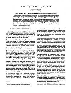
Let G = (V, E) ∈ G and fix a local edge labeling f = {fv | v ∈ V }. Let v1 , . . . , vd be the vertices adjacent to v, where d = deg(v) is the degree of v. Definition 1 The view of G from v under f , Tf (v), is an infinite, labeled, rooted tree, defined recursively as follows. Tf (v) has the root x0 corresponding to v. For each vertex vi adjacent to v in G, Tf (v) has a node xi and an edge from x0 to xi with labels fv (v, vi ) and fvi (v, vi ) at its x0 ’s and xi ’s ends, respectively. Node xi is now the root of Tf (vi ) from vi . 2 6

z5

z4

z3

z6

z6 z1

z2

Figure 1: Definition of view Tf (v) from v under f . In the above definition, x0 and xi are used for definition purposes only and not part of the view. (See Figure 1.) Note that the nodes of Tf (v) come from V , but they are not labeled as such. For example, xi in the above definition is a local name known only to processor v and it is not labeled by vi . But an algorithm (executed at a processor) can sometimes reveal the true identity, i.e., vi , of a node of Tf (v), as will be discussed below. The view Tf (v) represents the set of all infinite walks in G starting at v, with port numbers appearing along each walk. To avoid confusion, in the rest of the paper, the vertices of a view will be referred to as nodes, to distinguish them from the vertices of networks under consideration. u, v and w (with or without subscripts) will denote vertices, and x, y and z (with or without subscripts) will denote nodes, unless otherwise stated. If x denotes a node of a view, then x ∈ V denotes the corresponding vertex of G. Example 1 Consider the network G given in Figure 2(a). The integers attached to the edges in the figure present a local edge labeling f for G. Figure 2(b) illustrates the view, Tf (u2 ), from u2 , which is constructed as follows. Starting with the root node x0 , we draw an edge (x0 , x1 ) with labels 3 and 1 corresponding to the walk from u2 to u1 in G. We thus have x0 = u2 and x1 = u1 . Similarly, we draw (x0 , x2 ) with labels 1 and 1 corresponding to the walk from u2 to u3 . The edge (x1 , x4 ) with labels 1 and 3 corresponds to the walk from u1 back to u2 in G, and so forth. Note that labels 1 and 3 are attached in this order, since this time the edge (u2 , u1 ) is traversed from u1 to u2 . Observe that Tf (u2 ) is an infinite tree, and the three subtrees of its root are, from left to right, Tf (u1 ), Tf (u3 ) and Tf (u4 ). Tf (u2 ) and Tf (u4 ) also appear as subtrees of Tf (u3 ). 2 Clearly, the edge label sequences along different walks starting from the root of Tf (v) are distinct. Therefore, there is a one-to-one correspondence between the nodes of Tf (v) and the label sequences, from the root to those nodes. Let T be a view, and let P (T, x) denote the shortest path connecting the root and node x in T , and let L(T, x) denote the sequence of edge labels (two per edge) along P (T, x). Recall that vi ’s are not shown in Tf (v) and that the correspondence between P (T, x) and L(T, x) is one-to-one. 7

u4

1 2 2

u2 u1

3

1

1

2 u3

1 (a) x0 3

2 1

1

1

x1

x2

1

1

3 x4

2

1

2

1

u2

x3 2

2 x7

x6

x5

u2

1

u4

2 x8

u2

u3

(b)

Figure 2: An example of a view. (a) A graph G; (b) Tf (u2 ). Two views T and T ′ are said to be similar , written T ≡ T ′ , if there is a graph isomorphism between them which preserves the root and edge labels. It is easy to see that ≡ is an equivalence relation. Note that there may be many vertices v in V having similar views. Let Tf denote the set of all dissimilar views, i.e., Tf = {Tf (v) | v ∈ V } with one representative from each equivalence based on similarity. We may omit f from Tf (v) and Tf , whenever it is obvious from the context. Lemma 1 Let f be a local edge labeling of a network G, and let ui and uj be any two distinct vertices such that Tf (ui ) ≡ Tf (uj ). Consider any two paths P (T (ui ), zi ) and P (T (uj ), zj ) in T (ui ) and T (uj ), respectively, such that the two label sequences L(T (ui ), zi ) and L(T (uj ), zj ) are identical. Then T (zi ) ≡ T (zj ) and zi 6= zj holds. Proof Consider two paths, πi and πj , in G corresponding to P (T (ui ), zi ) and P (T (uj ), zj ). They start at vertices ui and uj and end at vertices zi and zj , respectively. We assume 8

T (zi ) 6≡ T (zj ) and derive a contradiction. If T (zi ) 6≡ T (zj ), then without loss of generality there is a path π in G starting at zi such that there is no path starting at zj having the same label sequence as π. This means that T (ui ) has a walk corresponding to πi π, but T (uj ) doesn’t have a walk corresponding to πi π, a contradiction. Now, to prove the second assertion of the lemma, assume that zi = zj for some i 6= j, and without loss of generality let P (T (ui ), zi ) and P (T (uj ), zj ) be the shortest paths such that zi = zj . Then, in G, the walk from ui to zi and that from uj to zj have the same label sequence and meet at zi = zj . This is impossible, since the ports of zi at which these walks end have different port numbers. 2 Corollary 1 The cardinality of the set {v | T (v) ≡ T } is the same for all T ∈ Tf . Proof Suppose that T (u) 6≡ T (v) for some u and v, and assume without loss of generality that the number of vertices having views similar to T (u) is greater than that of those having views similar to T (v). Let let u1 (= u), u2 , . . . , uk be distinct vertices such that T (u1 ) ≡ . . . ≡ T (uk ). Since G is connected, there exists a path P (T (u), z), where z is a node such that z = v. For each i = 1, 2, . . . , k, define a node zi of T (ui ) by L(T (ui ), zi ) = L(T (u), z). Note that zi is uniquely determined. By Lemma 1, we have T (zi ) ≡ T (zj ) and zi 6= zj for any 1 ≤ i, j ≤ k, a contradiction to the above assumption. 2 For any local edge labeling f for a graph with n vertices, we define sf by sf = n/|Tf |, where |Tf | denotes the cardinality of Tf . Corollary 1 implies that sf is an integer, and that sf is the cardinality of the set {v | T (v) ≡ T } for any T ∈ Tf . For the example of Figure 2(a), sf = 1, since no two views are similar, as easily checked by examining Figure 2(b). For any positive integer d, let #d (G) denote the number of vertices of G with degree d. Clearly, #d (G) = 0 for all d ≥ n. Since two vertices with different degrees cannot be similar under f , we have the following. Proposition 3 1. For any graph G and any local edge labeling f for G, sf divides the size n of G. 2. sf also divides #d (G) for each d = 1, 2, . . . , n − 1.

2

Based on Corollary 1, we now introduce an important property, called symmetricity, of a graph. Definition 2 The symmetricity of a graph G is defined by σ(G) = max{sf | f is a local edge labeling for G}. 2

9

Intuitively, Tf (v) represents the maximum information that processor v can obtain in the worst case (i.e., under the most unfavorable communication timing) by exchanging messages with others. Therefore, the larger the number of processors which have similar views, the more difficult it is to identify their accurate positions in G. The symmetricity σ(G) indicates, in the worst case (i.e., under the most unfavorable labeling), how many processors have similar views. Proposition 3 implies that σ(G) divides the size n of G, since σ(G) = sf for some f . Lemma 2 For any two local edge labelings f and g, if Tf ∩ Tg 6= ∅, then Tf = Tg . Proof Let T ∈ (Tf ∩ Tg ) 6= ∅ and let v and w be vertices in V such that Tf (v) ≡ Tg (w) ≡ T . We assume Tf 6= Tg and derive a contradiction. Without loss of generality, we can assume that there exists a vertex u in V such that Tg does not contain Tf (u). Since G is connected, there exists a path P (Tf (v), z) connecting the root of Tf (v) and a node z, satisfying u = z. Since Tf (v) ≡ Tg (w), there exists a node z ′ in Tg (w) such that P (Tf (v), z) = P (Tg (w), z ′ ) and the subtree of Tg (w) rooted at z ′ is similar to the subtree of Tf (v) rooted at z, a contradiction. 2 Intuitively, the above lemma implies that any element of Tf carries all the information about Tf . For any integer d ≥ 0, let T d (v) denote T (v) truncated to depth d, where depth is the distance (in the number of edges) from the root. We assume that each leaf of T d (v) contains the number of children the corresponding node in T (v) has. The following lemma is by Norris[27]. Lemma 3

3.2

8

T (u) ≡ T (v) if and only if T n−1 (u) ≡ T n−1 (v).

2

Pseudo–Synchronous Algorithms

The main objective of this subsection is to prove that, roughly speaking, the view from a vertex contains all the information that a distributed algorithm can possibly use (Lemma 5), and therefore, in the light of Lemma 3, the sole purpose of message exchanges is to construct a finite view at each vertex. Lemma 4 Given any network G, there is an algorithm for each processor v on G to construct T d (v) for any given nonnegative integer d. Proof We give a sketch of a simple algorithm for each processor v to construct T d (v). Let T0 (v) be the trivial tree consisting only of the root with information deg(v); for i = 0 to d − 1 do { Send a message (T i (v), j) via port j = 1, 2, . . . , deg(v); Wait until a message has been received from each port j = 1, 2, . . . , deg(v); Construct T i+1 (v) using the available information; } od 8

We originally proved the the following fact[36], which was recently improved by Norris: 2

2

T (u) ≡ T (v) if and only if T n (u) ≡ T n (v).

10

It is easy to show that the above algorithm is correct.

2

Note that only the leaves of the received trees (and their incident edges) contain new information needed to extend T i (v) to T i+1 (v). Alternatively, v can discard T i (v) and construct T i+1 (v) by attaching the received trees to a single node (the root). Since processor v does not know that its identity number is v, neither does it know that the view it produces is T d (v). We now define a phase of an algorithm as the following sequence of instructions. • If the termination condition holds, send message done via each port j and terminate; • Send messages via some ports (at most one per port); • Send message end-phase via each port j; • Receive messages until exactly one done or end-phase message is received from each port j via which no done message has been received in an earlier phase; • Process information in its local memory; An algorithm is called pseudo-synchronous if it consists of phases. Number the phases of a distributed pseudo-synchronous algorithm, 1, 2, . . . , from the initial phase onwards. Clearly, if the shortest distance (in terms of the number of links) between two processors is d, then it takes d phases for information to travel from one to the other. Let A be an algorithm for solving a problem P . The execution of A on a processor consists of an interleaved sequence of processing activities and message exchanges. If, during a round of message exchanges, A does not send any message via some ports, modify A to send an end-phase message via each of those ports. Then, it can also expect to receive a message from each port. The resulting algorithm will be pseudo-synchronous. We thus have the following fact. Proposition 4 For any network G ∈ G, there is an algorithm for solving a problem P on G, if and only if there is a pseudo-synchronous algorithm for solving P on G. 2 The following lemma will form a basis of our subsequent discussions. Its implications are it is possible that any two processors having similar views behave in precisely the same way and, therefore, the labeling which labels each processor by its view is a similarity labeling (see [17]). Lemma 5 Let P ∈ P and G ∈ G. There is an algorithm A for solving P on G, using some network attribute information I about G (e.g., size, topology, upbound), if and only if there is a pseudo-synchronous algorithm B for solving P on G using I, such that, in each phase p + 1 (p ≥ 0), each processor v sends Tfp (v), and nothing else, to all its neighbors. Proof The if part is trivial, so we concentrate on the only if part. By Proposition 4, we can assume without loss of generality that algorithm A is pseudo-synchronous. The essential assertion of this lemma is that all information that A, running on processor v, exchanges in its phase p + 1 is contained in Tfp (v). Therefore, we need to show that algorithm B can simulate A using only the information contained in Tfp (v). 11

We first describe how, for any phase p of A, algorithm B, running on processor v, can determine the state of A’s execution at v at the end of phase p, if B has a copy of A, information I, and Tfp (v) at its disposal. Algorithm B simulates A’s phases 1 through p with the help of Tfp (v) as follows. Note that the state of A’s execution at v at the end of phase p depends on the messages sent by the vertices at distances up to p from v. Therefore, B simulates phase p of A using p rounds. In the first round, for each node x in Tfp (v), B simulates the phase 1 of A running on x. In this simulation, x follows the steps of A, simulating the sending/receiving of messages via each port, and then doing some computation. The root of the tree, in particular, is now in the same state that A, running on v, would be in at the end of phase 1. Algorithm B now proceeds to round i = 2, 3, . . . , p of simulation of A on x for each node x at distances ≤ p − i+ 1 from the root in Tfp (v). After p rounds of simulation, the root of the tree will be in the same execution state that A running on v would be in at the end of phase p. Algorithm B repeats the above simulation for each phase p = 1, 2, . . . , of A. Namely, B constructs Tfp (v) using the messages Tfp−1 (u) sent from each neighbor u (except when p = 1, in which case Tf0 (v) is locally available), and simulates A for the first p phases. If A does not terminate in phase p, B sends Tfp (v) to every neighbor in the next phase p+1. B eventually terminates since A does. 2 In the following several sections, we will investigate the classes of graphs for which the problems defined in Section 1 are solvable, applying the concept of graph symmetricity introduced in this section.

4

The Known Topology Case

We start our case study with topology. Since the topology is assumed to be known, an algorithm AG , specific to a particular network G on which it runs, will also be considered in this section. Recall, however, that each processor knows neither its identity number nor which vertex of G it is represented by. An algorithm must work correctly for any local edge labeling, since, by definition, it cannot expect any particular local edge labeling. The results of Subsections 4.1 and 4.2 apply equally well to size, where only the graph size n, not the topology, of the network is known. In view of Lemma 3, in the rest of this section, we define d = n − 1, and let Tfd denote the set of all dissimilar (partial) views Tfd (v), i.e., Tfd = {Tfd (v) | v ∈ V }. Note that Lemma 3 implies |Tfd | = |Tf |.

4.1

Characterization of Dtopology (ELECT-LEADER)

Lemma 6 A graph G is in Dtopology (ELECT-LEADER) if σ(G) = 1. Proof We give a sketch of an algorithm AEL for solving ELECT-LEADER. Since the set of all views truncated to finite depths is enumerable, we can fix a total order < among these finite views. AEL contains a subalgorithm for sorting a given finite set of finite views in the order σ(G) by Lemma 10, a contradiction to the definition of symmetricity. Only if part: Let g be the smallest integer such that G satisfies the F–condition with g. Then σ(G) ≥ n/g holds, since there is a local edge labeling f for G such that sf ≥ n/g by Lemma 10. To show σ(G) ≤ n/g, assume that σ(G) > n/g. Let f be a local edge labeling for G such that σ(G) = sf > n/g holds. Then by Corollary 3, G satisfies the F–condition with n/sf < g, a contradiction. 2 We now proceed to the problem of characterizing the set S of all trees. To this end, we first characterize cycles in G in terms of the structure of G/f .

20

Lemma 11 A graph G has a cycle if, for any local edge labeling f , G/f has one of the following: 1. a self-loop (Ti , Ti : p, q), (p 6= q), 2. two self-loops, (Ti , Ti : p, p) and (Tj , Tj : q, q), where p = q is not excluded if i 6= j, or 3. a cycle of length ≥ 2. Proof (I) Let e = (Ti , Ti : p, q) be a self-loop in G/f . By Lemma 9, τf−1 (e) is a 2–factor in GVi . Therefore, G has a cycle. (II) Let e = (Ti , Ti : p, p) and e′ = (Tj , Tj : q, q) be two self-loops. If they are at the same vertex Ti = Tj of G/f , then clearly, each vertex in the subgraph of G, F = (Vi , τf−1 (e) ∪ τf−1 (e′ )), has degree 2, hence F contains a cycle. If e and e′ are at two different vertices, then let F = (Vi //Vj , τf−1 (e) ∪ τf−1 (e′ )). Now, pick a spanning tree of G/f and construct a partition U1 , . . . , Usf , as in Theorem 4. In F , introduce sf new edges between Vi and Vj such that u ∈ Vi and v ∈ Vj are joined by an edge if and only if u, v ∈ Uh for some h. Such an edge indicates the fact that there is a path between u and v in the spanning tree in GUh . It is easy to see that this new graph, F ′ , has a cycle, since each vertex in it has degree 2. It follows that G has a cycle. (III) Let C be a cycle in G/f , and construct a spanning tree S of G/f so that all but one edge e = (Ti , Tj ) of C belong to S. Let F = (Vi //Vj , τf−1 (e)) and add sf new edges between Vi and Vj as in (II) above. The rest of the proof is analogous to (II). 2 The above lemma holds even if “if, for any local edge labeling f for G,” is replaced by “if there is a local edge labeling f for G such that”. In which of the three forms a cycle in G manifests itself in G/f depends on f . Theorem 6 A graph G is a tree if and only if, for any11 local edge labeling f for G, the quotient graph G/f = (Tf , Ef ) is a tree, except for at most one self-loop e = (Ti , Ti : p, p) for some Ti ∈ Tf and p. Proof The only if part follows directly from Lemma 11. To prove the if part, let G/f = (Tf , Ef ), where Tf = {T1 , . . . , Tg }, be a tree, except possibly for one self-loop. We try to reconstruct G = (V, E). V consists of g subsets V1 , . . . , Vg , corresponding to vertices T1 , . . . , Tg , of G/f . There are two cases to consider. (a) G/f has no self-loop. So G consists of sf disjoint trees. Since, by definition, G is connected, sf = 1 must hold. (b) G/f has a self-loop e = (Ti , Ti : p, p). Let S = (Tf , Ef −{e}) be the unique spanning tree of G/f , and consider the graph G′ = (V, E ′ ), where E ′ = {τf−1 (e′ ) | e′ ∈ Ef −{e}}. G′ is clearly a collection of sf (= n/g) disjoint trees, each isomorphic to S. The only difference between G and G′ is that the edges in τf−1 (e) are missing in G′ . By Lemma 9, F = (Vi , τf−1 (e)) is a 1–factor of GVi , which implies that each edge in τf−1 (e) joins a pair of trees in G′ . Therefore, sf is even and G consists of sf /2 disjoint trees. Since G is connected, we have sf = 2. In either case, G is a tree.

2

11

This theorem is valid even if “if, for any local edge labeling f for G,” is replaced by “if there is a local edge labeling f for G such that”.

21

5.2

Minimum Realization of a Quotient Graph

As we have seen, for any simple graph G′ and a local edge labeling f ′ for G′ , the quotient graph G′ /f ′ is a connected (not necessary simple) graph with edge labels. We extend the definition of local edge labeling to non–simple graphs by allowing the same port numbers at both ends of a self-loop. Thus the edge labels on a quotient graph G′ /f ′ form a local edge labeling. The problem we address in this subsection is: given a quotient graph Q = G′ /f ′ , construct a simple, connected graph G = (V, E) and a local edge labeling f , called a realization of Q, such that G/f is isomorphic to G′ /f ′ , including the edge labels. In general, there are many different realizations. For example, two different realizations of G/f shown in Figure 6(c) are given in Figures 6(a) and (b). A realization R = (G, f ) of G′ /f ′ is said to be minimum if G has the minimum number of vertices among all the realizations of G′ /f ′ . We restrict Q to the quotient graphs, since otherwise G/f may be smaller than Q for some “realizations” of Q.

2

1

1 2 3 1

1

2

1 2

2

2

2

1 3

3 2

2

1

1 3

1

2

1 2

2

1

1

(b)

(a)

1 2

2 1 3 1

1 2 (c)

Figure 6: Two graphs and their quotient graph: (a) G with f . (b) G′ with f ′ . (c) G/f is isomorphic to G′ /f ′ including the edge labels. Given a quotient graph Q = G′ /f ′ = (W, A), where W = {w1 , . . . , wg }, for each wi ∈ W , define three parameters, ℓi , mi and m ˆ i , as follows: • ℓi : the number of self-loops of the form (wi , wi : p, p) for some wi and p, • mi : the number of self-loops of the form (wi , wi : p, q) for some wi and p, q (p 6= q). • m ˆi = maxj(6=i) {mij }, where mij is the number of parallel edges connecting wi and wj . Define further m = max {1+ℓi +2mi , m ˆi }, wi ∈W

22

(1)

and M=

(

m if m is even or ℓi = 0 for all wi ∈ W, m + 1 otherwise.

We now want to determine the size of (i.e., the number of vertices in) the minimum realization. Note that, by Theorem 4, any realization (G, f ) of Q has sf |W | vertices. However, sf is a parameter of G, i.e., not G′ . Lemma 12 Given a quotient graph Q = G′ /f ′ = (W, A), every realization of Q has at least M |W | vertices. Proof Consider an arbitrary realization (G, f ) with size M ′ |W |, where G = (V, E). Let wi satisfy m = max{1 + ℓi + 2mi , m ˆi }, and let ψ be a label preserving isomorphism from ′ G/f to Q. We have |Vi | = M , where Vi = {v ∈ V | ψ(T (v)) = wi }. Since GVi contains ℓi 1–factors, it must have at least 1+ℓi vertices. Further, since GVi contains mi 2–factors, it must have at least 2mi additional vertices. Therefore, we have M ′ ≥ 1+ℓi+2mi . To see that M′ ≥ m ˆ i also holds, pick a particular j satisfying m ˆ i = mij . Then, by Lemma 9, BVi ,Vj = (Vi //Vj , E ∩ (Vi × Vj )) is a m ˆ i –regular bipartite graph, where Vj = {v ∈ V | ψ(T (v)) = wj }. We thus have M ′ ≥ m ˆ i . It follows that M ′ ≥ m. Also, if ℓi > 0 for some wi , M ′ must be even in order for a 1-factor to exist. Hence M ′ ≥ M . 2 The following theorem summarizes some known graph-decomposition results that we find useful in proving Lemma 13. Theorem 7 [15] 1. Any complete graph Kn of even size n is 1–factorable. 2. Any complete graph Kn of even size n is the sum of a 1–factor and (n−2)/2 spanning cycles. 3. Any complete graph Kn of odd size n is the sum of (n−1)/2 spanning cycles. 4. Any regular bipartite graph is 1-factorable.

2

Lemma 13 Given a quotient graph Q = G′ /f ′ = (W, A), there is a realization of Q which has M |W | vertices. Proof We construct a graph G = (V, E) with size M |W | and a local edge labeling f for G such that G/f is isomorphic to Q including the edge labels. Intuitively, we make M copies of each vertex wi of Q so that it is expanded into a set Vi of vertices of G. Theorem 7 states that the complete graph on M vertices has a sufficient number of vertices and edges to embed the {1, 2}–factorable regular graph corresponding to the set of self-loops at any vertex wi of Q (i.e., mutually edge-disjoint ℓi 1–factors and mi 2–factors). We embed the {1, 2}–factorable graph in the complete graph on Vi , and remove the remaining edges. Also, a complete bipartite graph on two sets of M vertices contains mutually edge disjoint m ˆ i 1–factors for any i. For each edge of Q between wi and wj , we introduce an edge set E ′ so that (Vi //Vj , E ′ ) is mij -regular bipartite. We give below a more formal construction. [MIN-LABEL] 23

Given a quotient graph Q = G′ /f ′ = (W, A) with |W | = g, prepare V = V1 ∪ V2 ∪ . . . ∪ Vg as a vertex set of G, where Vi ’s are pair-wise disjoint and |Vi | = M for each i = 1, . . . , g. For each edge (wi , wj : p, q) in Q, create a set of edges and define local edge labeling f as follows. Self-loops at wi : Let SL ⊆ A be the set of self-loops at wi ∈ W . (A) First consider the case ℓi = 0, i.e., |SL| = mi . Since M ≥ 1+2mi , by Theorem 7 the complete graph KM on Vi contains at least mi mutually edge disjoint spanning cycles. (If M is odd, apply Theorem 7 3., and if it is even, apply 2. to M ≥ 2+2mi .) For each edge (wi , wi : p, q) ∈ SL, we use a distinct spanning cycle F = (Vi , EF ) selected from them, and include EF in E. Local edge labeling f for EF is defined in such a way that labels p and q appear alternately along the cycle. More formally, let e0 , e1 , . . . , eM −1 (eh = (uh , uh+1 ), h = 0, 1, . . . , M −1) be the spanning cycle, where uM = u0 . Then define fuh (uh , uh+1 ) = p and fuh+1 (uh , uh+1 ) = q for h = 0, 1, . . . , M −1. (B) Suppose that ℓi > 0. Then M is even by definition. By Theorem 7, in this case, the complete graph KM on Vi contains a 1–facotor and (M − 2)/2 spanning cycles, which are mutually edge disjoint. For each edge (wi , wi : p, q) ∈ SL such that p 6= q, use a distinct spanning cycle F = (Vi , EF ) selected from the (M−2)/2 spanning cycles, and include EF in E. Then define local edge labeling f for EF as in Case (A). Since M ≥ 1+ ℓi + 2mi , the worst case is M = 1+ ℓi + 2mi , in which case ℓi is odd and (M − 2)/2 = (ℓi − 1)/2 + mi . Since we have used mi spanning cycles so far, there still remain (ℓi − 1)/2 spanning cycles and one 1–factor, which translate to ℓi mutually edge disjoint 1–factors. For each edge (wi , wi : p, p), we use a distinct 1– factor F = (Vi , EF ) selected from these 1–factors. (If ℓi ≥ 2, then use at least one pair of 1–factors which belong to the same spanning cycle, to make G connected.) Then include EF in E, and define local edge labeling f for EF as follows: For each e = (u, v) ∈ EF , fu (e) = fv (e) = p. Parallel edges (wi , wj ): Consider the complete regular bipartite graph KVi ,Vj , and select an arbitrary spanning cycle in it. By Theorem 7 4., the remaining edges can be decomposed into M − 2 1–factors. Decompose the spanning cycle into two 1–factors, F1 and F2 . Since M ≥ mij , for each edge (wi , wj : p, q), we can use a distinct 1–factor F = (Vi //Vj , EF ) from the M 1-factors. Include EF in E. (If mij ≥ 2, use both F1 and F2 for some edges to make G connected.) Define a local edge labeling f for EF as follows: For each e = (u, v) ∈ EF , fu (e) = p and fv (e) = q. [End of MIN-LABEL] It is easy to check that the graph G constructed by MIN-LABEL contains neither selfloops nor parallel edges. Also, if G is connected, it is easy to show that G/f is isomorphic to Q including the edge labels. In the rest of the proof, we show that G is always connected. Clearly, G is connected if Gi = GVi is connected for some i = 1, . . . , g, since each copy of Q is connected. Therefore, suppose that none of {Gi | i = 1, . . . , g} is not connected. By the construction MIN–LABEL, Gi is clearly connected if ℓi ≥ 2 or mi ≥ 1. Hence ℓi ≤ 1 and mi = 0 for all i. Also, G is connected if Gij = (Vi //Vj , E ∩ (Vi × Vj )) is connected for some pair of indices, i, j = 1, . . . , g, (i 6= j), since Q is connected. By the construction MIN-LABEL again, Gij is connected if mij ≥ 2. Hence, mij ≤ 1 for all i and j, which implies that m ˆ i = 1 for every i. 24

If ℓi = 0 for all i, then M = 1 and G is clearly connected. If ℓi = 1 for some i, then M = 2 and two vertices in Vi are connected, because of the 1–factor created in Gi ; hence G is connected. 2 Theorem 8 The minimum realization of Q = G′ /f ′ = (W, A) has size M |W |. Proof Follows from Lemmas 12 and 13.

2

Theorem 9 A graph G is a tree if and only if, for any local edge labeling f , all realizations of the quotient graph G/f are isomorphic (including the edge labels), i.e., for any two realizations (G1 , f1 ) and (G2 , f2 ) of G/f , there is a label-preserving isomorphism. Proof Only if part: Let G be a tree and f be a local edge labeling for G. We show that all realizations of the quotient graph G/f are isomorphic including the edge labels. By Theorem 6, G/f is a tree, except possibly for one self-loop. The proof of Theorem 6 shows that sf ≤ 2 and that sf = 2 if and only if G/f has a self-loop. First we examine the case sf = 1. In this case, G/f is clearly isomorphic (including the edge labels) to (G, f ). Suppose that there is a realization (G′ , f ′ ) which is not isomorphic to (G, f ), such that G′ /f ′ is isomorphic to G/f . Then cf ′ > 1, since otherwise (G′ , f ′ ), which is isomorphic to G′ /f ′ , would be isomorphic to G/f . Thus G′ /f ′ is not connected (see the proof of Theorem 6); therefore, (G′ /f ′ , f ′ ) cannot be a realization. If sf = 2, on the other hand, G/f is a tree except for one self-loop labeled (p, p) for some p. Let (G′ , f ′ ) be a realization of G/f . Again, using the proof of Theorem 6, we have cf ′ = 2. From the structure of G/f (i.e., a tree except for one self-loop corresponding to a 1–factor), (G′ , f ′ ) is uniquely determined. Therefore, (G′ , f ′ ) is isomorphic to G/f If part: Suppose that G is not a tree. We want to show that there are two realizations of G/f , (G1 , f1 ) and (G2 , f2 ), that are of different sizes and hence not isomorphic to each other. Let (G1 , f1 ) be the minimum realization of size M |W | known to exist by Theorem 8. Using any even number M ′ (> M ) instead of M in MIN-LABEL, we construct (G2 , f2 ) (which may not be connected) of size M ′ |W |, such that G2 /f2 is isomorphic to G/f . It remains to show that this (G2 , f2 ) is indeed a realization of G/f , i.e., it is connected. As in the proof of Lemma 13, we can make G2 connected when either ℓi ≥ 2, mi ≥ 1 or m ˆ i ≥ 2 holds for some i, where ℓi , mi , and m ˆ i are the parameters of G/f . So, we consider the remaining cases, in which ℓi ≤ 1, mi = 0 and m ˆ i ≤ 1 hold. Since G is not a tree, there is a local edge labeling f such that G/f does not satisfy the condition of Theorem 6. Thus, G/f must contain either (1) a cycle, or (2) two or more self-loops (but at most one at a given vertex since ℓi ≤ 1). In case (2), we have ℓi = 1 for some i, hence M ≥ 2, which implies M ′ ≥ 4. Let Q′ be the graph obtained from Q = G/f = (W, A) by removing any two self-loops e = (wi , wi : p, p) and e′ = (wj , wj : q, q), and let (G′2 , f2′ ) be the result of applying MIN-LABEL to Q′ . Each vertex set Vk used in MIN-LABEL has size M ′ . We obtain (G2 , f2 ) from (G′2 , f2′ ) by adding a 1–factor of Vi representing e and a 1–factor of Vj representing e′ . By Theorem 7 2., the complete graph on Vi has at least (M ′ − 2)/2 ≥ 1 spanning cycles (call one of them Ci ). Similarly, the complete graph on Vj has at least one spanning cycle (call it Cj ). Ci (Cj ) can be decomposed to two 1-factors, of which we use one to represent e (e′ ). To make the resulting G2 connected, we need a certain relationship between Ci and Cj . Let U1 , U2 , . . . , Ug be the sets defined for G′2 /f2′ by Theorem 4. Without loss of generality, we assume 25

that each edge of Ci connects a vertex of Uk to a vertex of Uk+1 , for some k = 1, 2, . . . , g, where Ug+1 = U1 . Similarly for Cj . The 1–factor of Ci we use to represent e consists of the edges Ci connecting a vertex in Uk to a vertex in Uk+1 , for k = 1, 3, . . . , while the 1–factor of Cj we use to represent e′ consists of the edges of Cj connecting a vertex in Uk to a vertex in Uk+1 , for i = 2, 4, . . . It is easy to see that the resulting G2 is connected. In case (1), let e(wi , wj ) be an edge on a cycle C in G/f = (W, A). Apply MIN–LABEL to (W, A−{e}) to construct (G′2 , f2′ ) of size M ′ |W |. To convert (G′2 , f2′ ) into (G2 , f2 ), we apply the step for the parallel edges of MIN-LABEL, using a 1–factor in KVi ,Vj . This 1–factor can be so chosen that the resulting G2 is connected. 2 Corollary 4 A graph G is a tree if and only if the following condition holds for any labeling f : For any two realizations (G1 , f1 ) and (G2 , f2 ) of G/f , G1 ≃ G2 . 2 Proof The only if part follows from Theorem 9. The if part follows from the if part proof of Theorem 9. 2 It might appear that any non-tree graph G with σ(G) = 1 would also have the property of Theorem 9, since G/f has neither self-loops nor parallel edges. However, it turns out that this is not the case. Consider, for example, the graph G and local edge labeling f for G shown in Figure 2(a). Then σ(G) = 1, but the graph G′ and the local edge labeling f ′ for G′ shown in Figure 7 form another realization of G/f (= G) that is not isomorphic to G. 2

2

1 1

1

3 2

1

1

2 1

2

2

3

1

1

Figure 7: A realization of G = G/f of Figure 2(a).

6

Networks without Topology Information

In this section, we investigate networks G under the assumption that the processors running on G do not know the topology of G. In Subsection 6.1, we assume that the processors do know the size (i.e., the number of vertices) n of G, while in Subsection 6.2, we investigate model in which the processors only know an upper bound on n. Finally, in Subsection 6.3, computing under noinfo is investigated. In Subsections 6.1 and 6.2, the following theorem will play an important role. Theorem 10 For any graph G and local edge labeling f for G, there is an algorithm A ∈ ALG upbound for constructing G/f . Proof Let n be an upper bound on the size n of G. A can construct Tfn−1 as in the proof of Lemma 6. By Lemma 3, A can thus construct the vertex set Tf of G/f . Its edge set can 2 also be constructed from Tfn−1 . 26

If an upper bound on the network size is known, then, by Theorem 10, we can assume without loss of generality that each processor knows the quotient graph G/f for the given local edge labeling f . Thus the difference between results in Section 4 and the corresponding results in subsections 6.1 and 6.2 are due to the difference in the information that the processors are given or can compute; in Section 4, the processors knew G, while in Subsections 6.1 and 6.2, they can know only G/f . For a problem P and an algorithm A, recall the definition of N (P, A) given in Section 2. Let I ∈ {topology, size, upbound, noinfo}. In general, an algorithm A for solving problem P may actually solve P regardless of the local edge labeling only on a subset of networks in DI (P ). For the other networks in DI (P ), A may either solve P or report that it cannot solve P on the network it is running on with the given local edge labeling. A is said to be universal for DI (P ), if N (P, A) ⊇ DI (P ).12

6.1 6.1.1

Computing with a Known Number of Processors ELECT-LEADER, ELECT-EDGE, and SPANNING-TREE

The algorithm AEL (resp. AEE ) used in the proof of Lemma 6 (resp. Theorem 2) belongs to ALG size (⊃ ALG topology ) and solves ELECT-LEADER (resp. ELECT-EDGE) on any graph in Dtopology (ELECT-LEADER) (resp. Dtopology (ELECT-EDGE)).13 This implies that for P = ELECT-LEADER and ELECT-EDGE, Dsize (P ) = Dtopology (P ) and that AEL (resp. AEE ) is universal for Dsize (ELECT-LEADER) = Dtopology (ELECTLEADER) (resp. Dsize (ELECT-EDGE) = Dtopology (ELECT-EDGE)). It turns out that SPANNING-TREE also shares the same property, as asserted by the next theorem. Theorem 11 For problem P = ELECT-LEADER, ELECT-EDGE, and SPANNINGTREE, there is an algorithm AP ∈ ALGsize such that AP is universal for Dtopology (P ).

Proof Algorithms AEL and AEE provide a proof for P = ELECT-LEADER and ELECTEDGE, respectively. Consider the case P = SPANNING-TREE. We give a sketch of an algorithm AST satisfying the conditions of the theorem. AST first invokes AEE on the given (G, f ). When AEE finds that it cannot elect an edge in (G, f ), AST generates an output stating that it cannot solve SPANNING-TREE on (G, f ). Otherwise, AEE elects an edge. Let u and v be the two end vertices of the elected edge. Then on u and v, AST invokes the single-source-edge spanning tree algorithm SE–ST described in the proof of Theorem 3, and constructs a spanning tree. Note that SE-ST requires no network attribute information. It is clear that AST satisfies the conditions of the theorem, since Dtopology (SPANNING-TREE) = Dtopology (ELECT-EDGE) by Theorem 3. 2 Since no algorithm can solve problem P for all possible local labelings on any graph not belonging to Dtopology (P ), algorithms AEL , AEE and AST are the best possible. 12

As stated in the footnote to Lemma 6, Algorithm A may be able to solve P for a network G 6∈ N (P, A) for particular (but not for all) local edge labelings. Thus, A may not be able to decide whether the network on which it is running is in DI (P ) or not. 13 For the characterizations of Dtopology (ELECT-LEADER) and Dtopology (ELECT-EDGE), recall Theorems 1 and 2.

27

Corollary 5 For any P ∈ {ELECT-LEADER, ELECT-EDGE, SPANNING-TREE}, Dsize (P ) = Dtopology (P ). 2 6.1.2

FIND-TOPOLOGY

The equality Dsize (P ) = Dtopology (P ) in Corollary 5 implies that, when size n is known, knowing G or G/f makes no difference for ELECT-LEADER, ELECT-EDGE, or SPANNINGTREE, as far as their solvable classes are concerned. However, as we se below, it does make an essential difference for FIND-TOPOLOGY. Lemma 14 If G ∈ Dsize (FIND-TOPOLOGY), then for any local edge labeling f for G the following holds: For any realization (G′ , f ′ ) of G/f , if G′ and G have the same size then we have G′ ≃ G.14 Proof Assume that there is an algorithm A ∈ ALGsize which solves FIND-TOPOLOGY on (G, f ), where G ∈ Dsize (FIND-TOPOLOGY) does not satisfy the condition of the lemma. We derive a contradiction out of this assumption. By Lemma 5, there is a pseudo synchronous algorithm B ∈ ALGsize for solving FIND-TOPOLOGY on (G, f ) such that, in each phase p+1 (p ≥ 0), each processor v sends Tfp (v), and nothing else, to every one of its neighbors. Let (G′ , f ′ ) be a realization of G/f such that G and G′ have the same size but G′ 6≃ G. Let B run on (G′ , f ′ ). Since G/f is isomorphic to G′ /f ′ including edge labels, and G and G′ have the same size, each processor, running B on (G′ , f ′ ), outputs (G, f ). This is a contradiction, since each processor should either output (G′ , f ′ ) or report that it cannot solve FIND-TOPOLOGY on the network it is running. 2 The following theorem is FIND-TOPOLOGY’s counterpart to Theorem 11. Note that Dsize (FIND-TOPOLOGY) 6= Dtopology (FIND-TOPOLOGY). Theorem 12 There is an algorithm ATR ∈ ALGsize which is universal for Dsize (FINDTOPOLOGY).15 Proof We give a sketch of an algorithm ATR for solving FIND-TOPOLOGY. Running on a graph G with n vertices with a local edge labeling f , ATR first computes G/f . Since ATR knows n and since the number of graphs with n vertices is finite, it can enumerate all the realizations (G′ , f ′ ) of G/f such that G′ has n vertices and check whether all G′ ’s are isomorphic. If they are isomorphic then ATR outputs any one of them. Otherwise, based on Lemma 14, its output states that the graph on which it is running is not in Dsize (FIND-TOPOLOGY). A’s universality, i.e., N (FIND-TOPOLOGY,ATR ) = Dsize (FIND-TOPOLOGY), follows from Lemma 14. 2 Corollary 6 The condition of Lemma 14 is necessary and sufficient for G to be in Dsize (FINDTOPOLOGY). 2 14

That two graphs G′ and G without edge labels are isomorphic is denoted by G′ ≃ G, as was defined in Section 5. 15 For all G ∈ / Dsize (FIND-TOPOLOGY), ATR reports that G is not solvable, regardless of the given local edge labeling. This should be contrasted to Theorem 11, recalling the definition of the universality of an algorithm.

28

Proof Follows from Lemma 14 and Theorem 12.

2

Based on the characterization of Dsize (FIND-TOPOLOGY) given by Corollary 6, the following theorem clarifies the inclusion relationship between Dsize (FIND-TOPOLOGY) and some other classes. Theorem 13 1. Dtopology (ELECT-LEADER) ∪ S ⊂ Dsize (FIND-TOPOLOGY). 2. Dtopology (ELECT-EDGE) and Dsize (FIND-TOPOLOGY) are incomparable. Proof (1.) By Theorem 9 and Corollary 6, we have S ⊂ Dsize (FIND-TOPOLOGY). The fact Dtopology (ELECT-LEADER)⊂ Dsize (FIND-TOPOLOGY) follows from Theorem 1, Corollary 6, and from the fact that G is isomorphic to G/f (including the edge labels) for any f if σ(G) = 1. (2.) Consider the ring R3 on three vertices. Since σ(R3 ) = 3, we have R3 6∈ Dtopology (ELECTEDGE) by Theorem 2. However, R3 ∈ Dsize (FIND-TOPOLOGY) since it satisfies the condition of Lemma 14 (and by Corollary 6). Consider next the graph G shown in Figure 6(a). We have G ∈ Dtopology (ELECTEDGE) by Theorem 2. However, we can show that G 6∈ Dsize (FIND-TOPOLOGY), using Corollary 6. To see this, consider the labeling f for G shown in Figure 6(a). Figure 6(c) shows G/f . There is another realization of G/f , shown in Figure 6(b), which has the same size as G but is not isomorphic to G. 2 Theorem 14 Algorithms AEL , AEE , AST and ATR each have message complexity (i.e., the total number of messages exchanged in the worst case) O(nm), where m is the number of edges. 2(n−1)

Proof The majority of messages are needed to construct Tf be constructed with O(nm) messages.

6.2

2(n−1)

. By Lemma 4, Tf

can 2

Computing with an Upper Bound on the Number of Processors

Given a network G of size n, let n be an upper bound on n. If n−n ≤ 1, then knowing n is just as good as knowing n by Proposition 3. This is why we defined N (P, A) in Secton 2 as follows: For an algorithm A ∈ ALG upbound , N (P, A) is the set of networks G such that A can solve problem P for G, no matter how large an upper bound n on the size n of G is given. Theorem 15 For P = ELECT-LEADER, ELECT-EDGE, and SPANNING-TREE, there is an “algorithm” AP ∈ ALG upbound which is “universal” for Dtopology (P ).16 16

However, AP may fail to produce a valid output for a network not in Dtopology (P ). Strictly speaking, therefore, an “algorithm” here is not an algorithm in the sense defined in Section 2. Therefore, the term “universal” used in this theorem should also be interpreted mutatis mutandis. Therefore, this theorem is not used anywhere else in this paper.

29

Proof By Corollary 5, it is sufficient to show that, in each case, the exact size n is computable. Consider first the case P = ELECT-LEADER. Let G ∈ Dtopology (ELECT-LEADER) and let f be a local edge labeling for G. By Theorem 1, we have σ(G) = 1. By Theorem 10, each processor can compute G/f , based on an upper bound n on its size, and hence the exact size n = |G/f |.17 Next, consider the case P = ELECT-EDGE or SPANNING-TREE. Let G ∈ Dtopology (ELECT-EDGE) = Dtopology (SPANNING-TREE) (see Theorem 3) and let f be a local edge labeling for G. By Theorem 10, each processor can compute G/f , based on an upper bound n on its size. Note that, by Theorem 2, we have σ(G) ≤ 2, hence sf ≤ 2. If sf = 1 then G has the same size as G/f . If sf = 2, on the other hand, then G has exactly twice the size of G/f . The remaining problem is how to determine sf . We claim that sf = 1 if and only if G/f has no self-loops. By definition, the only if part is clear. To prove the if part, assume that sf = 2. Then σ(G) = 2, and by Theorem 2, there are adjacent vertices u and v such that T (u) ≡ T (v), which implies that there is a self-loop in G/f . 2 Theorem 16 Let S denote the set of all trees. We have: 1. Dupbound (FIND-TOPOLOGY) = S, 2. Dupbound (ELECT-EDGE) = Dupbound (SPANNING-TREE) = S, and 3. Dupbound (ELECT-LEADER) = Dtopology (ELECT-LEADER) ∩ S. Proof By Theorems 10 and 6, there is an algorithm in ALG upbound that can decide if the network with a local edge labeling, (G, f ), on which it is running is a tree and determine sf (1 or 2 by Corollary 2) or the number n of vertices if it is a tree. Once it is discovered that G is a tree, it is easy to solve any of the four problems using G/f . (As for ELECT-LEADER, if sf = 2, the algorithm reports that it cannot be solved for the tree.) It follows that S is contained in Dupbound (FIND-TOPOLOGY), Dupbound (ELECTEDGE) and Dupbound (SPANNING-TREE), and that Dtopology (ELECT-LEADER) ∩S is contained in Dupbound (ELECT-LEADER), since G ∈ Dtopology (ELECT-LEADER) if and only if σ(G) = 1 by Theorem 1. To prove that these inclusion relationships are really equalities, consider any network G∈ / S. By Theorem 9 and MIN-LABEL in the proof of Lemma 13, there exists a local edge labeling f for G such that, for any sufficiently large even number k, there is a realization (G′ , f ′ ) with cf ′ = k. Note that G/f is isomorphic to G′ f ′ including edge labels, but G′ 6≃ G in general. (I) To show that G ∈ / Dupbound (FIND-TOPOLOGY) for ∀G ∈ / S, we assume that there is an algorithm A ∈ ALG upbound such that G ∈ N (FIND-TOPOLOGY, A), and derive a contradiction. Let B be a pseudo synchronous algorithm for solving FIND-TOPOLOGY on G such that, in each phase p+1 (p ≥ 0), each processor v sends Tfp (v), and nothing else, to every one of its neighbors. Compare the computation of B on G with f and G′ with f ′ , assuming that a sufficiently large upper bound n is given as input data. Since Tf = Tf ′ , 17

Here, the processor is working on the assumption that σ(G) = 1, which is not valid, in general. See the previous footnote.

30

any two vertices having similar views, u in G and v in G′ , output the same answer, a contradiction. It follows that Dupbound (FIND-TOPOLOGY) ⊆ S, which proves (1.). (II) To show that G ∈ / Dupbound (ELECT-EDGE) for ∀G ∈ / S, assume that there is an algorithm A ∈ ALG upbound such that G ∈ N (ELECT-EDGE,A). By choosing k ≥ 3, we can make σ(G′ ) ≥ 3, which means G′ 6∈ Dtopology (ELECT-EDGE) by Theorem 2. Let B be a pseudo synchronous version of A (see Lemma 5) such that, in each phase p + 1 (p ≥ 0), each processor v sends Tfp (v), and nothing else, to every one of its neighbors. By the same argument as in (I) above, B can solve ELECT-EDGE for G′ , a contradiction since G′ 6∈ Dtopology (ELECT-EDGE). The fact that no non-tree network is in Dupbound (SPANNING-TREE) can be shown by a similar argument. (III) The proof for (3.) is analogous to (2.), except that Dupbound (ELECT-LEADER) ⊆ Dtopology (ELECT-LEADER) by Proposition 1. This additional condition is necessary because S is not contained in Dtopology (ELECT-LEADER). 2 Theorem 17 For any problem P ∈ P there is an algorithm A with message complexity O(nm) such that N (P, A) = Dupbound (P ), where n is the given upper bound on n. Proof Analogous to the proof of Theorem 14. (Replace n by n.)

6.3

2

Computing without Network Attribute Information

Theorem 18 For any problem P ∈ P, we have Dnoinfo (P ) = Dupbound (P ).

Proof For any graph G ∈ Dupbound (P )(⊆ S), we construct an algorithm AG ∈ ALG noinfo such that each processor on G′ solves P if and only if G′ is isomorphic to G; hence G ∈ N (P, AG ). All AG has to do is to recognize if network G′ is isomorphic to G (without any attribute information on G′ ), since P is solvable on G if G is known (because G ∈ Dupbound (P ) ⊆ Dtopology (P ) for ∀P ∈ P). Let G have n vertices. To explain the main idea behind AG , let us first reexamine view Tf (v), where v is a vertex of G′ and f is a local edge labeling for G′ . It consists of all paths in G′ originating at v. Each such path is infinitely long, and in general visits a vertex many times. Consider now the longest finite prefix of such a path, that is simple, i.e., does not visit any vertex more than once. (If G is a tree, in particular, then each such prefix ends at a leaf.) Moreover, the graph induced by the union of all such prefixes is exactly G′ . Once G′ is constructed, all that remains is to test if G′ is isomorphic to G. Running on G′ , AG first constructs Tfn (v) on each processor v, where n is the size of G. Note that what is stated in the previous paragraph is still valid if Tf (v) is replaced by Tfn (v), except that each path in Tfn (v) has finite length n. We now describe an easy way to determine the longest simple prefix of each path in Tfn (v). Let x and z be the parent and a child nodes of a node y in Tfn (v), respectively. Observe that x = z if and only if edges (x, y) and (y, z) are labeled by (p, q) and (q, p), respectively, for some p and q. Therefore, to determine the longest simple prefix of a path in Tfn (v), we truncate the path at the 31

first edge (y, z) on it satisfying the condition above for the parent node x of y. Call the resulting tree T ∗ . T ∗ ≃ G′ if T ∗ is “small” enough, or to be more precise, if T ∗ does not have a leaf vertex at depth n. If T ∗ has a leaf vertex at depth n, then AG reports that it gives up solving P for the network. Otherwise, since T ∗ ≃ G′ , it can invoke an appropriate algorithm (e.g., AEL ) in ALGtopology described in Section 4. (AG can simply output T ∗ if P = FIND-TOPOLOGY.) 2 The above theorem says that the upper bound information has no benefit, as far as the solvable classes are concerned. However, Theorem 19 below shows its effect on the existence of universal algorithms. To see the contrast more clearly, we first summarize what we already know about the cases where we do have some attribute information. Corollary 7 For any problem P ∈ P and any I in {topology, size, upbound}, there is a universal algorithm AP ∈ ALG I for DI (P ). 2 Theorem 19 For any problem P ∈ P, there is no universal algorithm A ∈ ALG noinfo for Dnoinfo (P ) (= Dupbound (P )).18 Proof Let R3 be the ring on three vertices and let f a local edge labeling for R3 such that each edge is labeled by (1, 2). Consider any algorithm A ∈ ALG noinfo for solving P . By Proposition 4, we can assume without loss of generality that A is pseudo synchronous. Since R3 is not a tree, by Theorem 16, no algorithm in ALG upbound , a fortiori, not A, can solve P on R3 . Therefore, the execution of A on R3 must terminate in the kth phase, for some integer k, announcing its inability to solve P on R3 . Lemma 5 implies that the execution of A on any processor v in any network G with any local edge labeling g would produce the same output as that on processor u in R3 , if Tfk (u) on R3 is similar to Tgk (v) on G. Let L be a “chain” graph with 2k+3 vertices, i.e., L = (V, E), where V = {v1 , v2 , . . . , v2k+3 } and E = {{vi , vi+1 } | i = 1, . . . , 2k+2}. Consider the labeling g for L such that all the edges are labeled by (1, 2) except for edge {v2k+2 , v2k+3 }, which has label (1,1). Clearly, Tfk (u) on R3 is similar to Tgk (vk ) on G. Thus L 6∈ N (P, A), although L ∈ Dupbound (P ) by Theorems 1 and 16. It follows that A is not universal. 2 Figure 8 illustrates the inclusion relationships among Dtopology (P ), Dsize (P ), Dupbound ( P) and Dnoinfo (P ), where P ∈ P.

7

Other Related Results

7.1

The Link Information

In Section 6, we investigated networks under the assumption that each processor knows the size n or an upper bound on n. We may also consider the case where each processor knows the number of links m or an upper bound on m, although this assumption may be a little artificial. 18

Therefore, for any algorithm A ∈ ALG noinfo for P , there is a network G such that P is not solvable on G by A, but is solvable by some other algorithm A′ ∈ ALG noinfo .

32

Lemma 15 Given a graph G with a local edge labeling f , let G/f = (W, F ). If G/f has s self-loops with the same label p at both ends, then m = sf (|F | − s/2).

Proof In Lemma 9, we considered three types of edges in F . For any edge e of type (1.), we showed there that sf = |V1 | = 2|τf−1 (e)|, while for any edge e of type (2.) or (3.), sf = |τf−1 (e)|. Therefore, an edge of type (1.) in G/f corresponds to sf /2 edges in G, while an edge of type (2.) or (3.) in G/f corresponds to sf edges in G. 2 For each problem P ∈ P let DEsize (P ) denote the set of networks for which P is solvable using m as an input. If each processor knows the number of vertices n, then it can construct G/f (see Theorem 10) and compute m by Lemma 15. Conversely, if it knows m, then it can construct G/f by Theorem 10, since m+1 is an upper bound on n if G is connected. It can then compute sf by Lemma 15 and obtain n = sf |W |. We therefore have the following theorem. Theorem 20 For each problem P ∈ P, we have DEsize (P ) = Dsize (P ). 2 Next, consider the case where the processors know an upper bound on m. Let DEupbound (P ) denote the set of networks for which P is solvable using an upper bound on m as input. The proof of the following corollary is analogous to the of the above theorem. Corollary 8 For each problem P ∈ P, we have DEupbound (P ) = Dupbound (P ). 2

7.2

Automorphisms

From the definition of symmetricity, it appears that there might be a close relation between the number of different automorphisms and the symmetricity of a graph (e.g., the larger the number of automorphisms, the larger the symmetricity would be, or there might be an automorphism if the symmetricity is greater than 1, and so on). Unfortunately, however, due to the following two properties, it turns out that there is no direct relation between the two quantities. A complete bipartite graph on two sets V1 and V2 , where |V1 | = 1, is called a star . An edge in a graph is called a bridge if its removal disconnects the graph. Proposition 5 1. Any star with at least 3 vertices has symmetricity 1; the number of automorphisms, however, increases with the number of vertices. 33

2. The symmetricity of any 3–regular bridge-less graph coincides with its size; however, there is a 3–regular bridge-less graph having no non-trivial automorphism. Proof 1. is easy to show. 2. follows from Theorem 5, since any 3–regular bridge-less graph is {1,2}–factorable [29]. 2 As for fixed-point-free automorphisms, we have the following result. Theorem 21 Let G be a graph with σ(G) = 2. Then, there is a fixed-point-free automorphism on G. Proof Let G = (V, E) and consider two distinct vertices u, v ∈ V such that Tf (u) ≡ Tf (v) for some local edge labeling f . Define a function ψ : V → V as follows. Let w ∈ V and x be a node of Tf (u) such that w = x. Then ψ(w) = y, where node y satisfies L(T (u), x) = L(T (v), y).19 Since G is connected, ψ is defined for every w in V . First, we show that ψ is a fixed-point-free function. Let x1 and x2 be any two nodes in T (u) such that w = x1 = x2 . Define y1 and y2 by L(T (u), x1 ) = L(T (v), y1 ) and L(T (u), x2 ) = L(T (v), y2 ), respectively. Since T (u) ≡ T (v) and x1 = x2 , the subtrees of T (v) rooted at y1 and y2 are similar. On the other hand, arguing as in the proof of Lemma 1, we can show that y1 6= w and y2 6= w since u 6= v. Hence, y1 and y2 must be the same since σ(G) = 2. Namely, ψ is a function and ψ(w) 6= w. Next, we show that ψ is an automorphism. Let e = (w1 , w2 ) ∈ E. Then, there are adjacent nodes x1 and x2 in T (u) such that x1 = w1 and x2 = w2 . Define two nodes y1 and y2 in T (v) by L(T (u), x1 ) = L(T (v), y1 ) and L(T (u), x2 ) = L(T (v), y2 ), respectively. Then 2 (ψ(w1 ), ψ(w2 )) = (y1 , y2 ) ∈ E, since y1 and y2 are adjacent.

7.3

Coverings

A graph K is said to be a covering of another graph G if there is a way to label the vertices of K with the names of vertices of G in such a way that, for each vertex u of K labeled v, the set of the labels of u’s neighbors in K coincides with the set of v’s neighbors in G. G and H are said to have a finite common covering if and only if there exists a graph K that is a covering of both G and H. Let G/f and H/g be two quotient graphs. If G/f is isomorphic to H/g including edge labels, then G and H have isomorphic universal coverings, where a universal covering of G is a (possibly infinite) tree which is a covering of G. Theorem 22 [2, 23] Two graphs G and H have a finite common covering if and only if they have isomorphic universal coverings. 2 Using the above theorem, a sufficient condition for a graph to be in Dsize (FINDTOPOLOGY), in terms of a common covering, can be derived. 19

L(T (u), x) was defined in Section 3.

34

Theorem 23 Let G be a graph. If there is no graph H with the same size as G such that G and H have a finite common covering, then G ∈ Dsize (FIND-TOPOLOGY). Proof We give a sketch of an algorithm A that solves FIND-TOPOLOGY for graphs satisfying the condition of theorem. When A is executed on a network G of size n under a local edge labeling f , it constructs the quotient graph G/f first, and then computes all pairs of a graph H of size n and a local edge labeling g such that H/g is isomorphic to G/f including edge labels. If all H’s are isomorphic, then A outputs H, otherwise, it gives up solving the problem. To show the correctness of A, suppose that A outputs a graph H of size n, which is not isomorphic to G. Since H/g is isomorphic to G/f including edge labels, H and G have isomorphic universal coverings, which implies that H and G have a finite common covering by Theorem 22, a contradiction. 2 Although the above sufficient condition is easier to understand than that of Lemma 14, unfortunately, it is not necessary. Any two r–regular graphs have a finite common covering since their universal coverings are isomorphic. Hence most of the regular graphs do not satisfy the sufficient condition; however, there are likely to be many regular graphs with symmetricity 1, which belong to Dsize (FIND-TOPOLOGY). Angluin [1] investigates a kind of topology recognition problem and shows that two graphs having a finite common covering are indistinguishable (Theorem 5.6 in [1]). This might appear to imply that the above sufficient condition would also be necessary. This is due to the difference between the FIND-TOPOLOGY and the recognition problem she investigates. Namely, her model assumes a more powerful communication mechanism than ours and the “coin tossing” facility which is not available in our model. G can be thought of as a kind of covering of G/f . As we have investigated in detail, the relation between G and G/f can be described in terms of p–factors. Thus some relation would exist between coverings and factors.

8

Discussions

ELECT-LEADER has been investigated by many researchers, mostly on networks with unique identity numbers. Rosenstiehl, Fiksel and Holliger showed that some problems are not solvable on symmetric graphs [31]. Borge has investigated “symmetry” and “genericity” of distributed systems and derived some necessary or sufficient conditions for ELECTLEADER to be solvable using these concepts [7, 8]. His model is based on CSP [16] and is closely related to Angluin’s. In his model, each process is aware of its (unique) name and, can use it in equality testing. As a tool to break symmetry, Itah and Rodeh use a probabilistic method [18], which is studied extensively for solving not only ELECT-LEADER but also other problems investigated in this paper (see, e.g., [22, 24, 33]). We have considered only connected networks. Johnson and Schneider [17] investigate a collection of disjoint networks. After extending the definition of ELECT-LEADER (“selection problem” in their terminology) to a collection of disjoint networks, they show that there is a similarity labeling algorithm for such a collection and, therefore, the extended ELECT-LEADER is decidable.

35

Let us extend the other three problems, ELECT-EDGE, SPANNING-TREE and FIND-TOPOLOGY, in the same way, and let P ′ denote the set of extended ELECTLEADER, ELECT-EDGE, SPANNING-TREE and FIND-TOPOLOGY. Thus, for each P ∈ P ′ , a solution must be found for each connected component of the network. We now briefly examine these extensions. Under topology, for any problem P ∈ P ′ , each processor can decide whether P is solvable for each connected component, using the topology information it has. Then, using AEL (see the proof of Lemma 6), AEE (see the proof of Theorem 2), or AST (see the proof of Theorem 11), each processor can solve P for the connected component to which it belongs. Solving FIND-TOPOLOGY is trivial. Thus we can conclude the following. For each problem P ∈ P ′ , there is a distributed algorithm in ALG topology which decides whether P is solvable for any given network and solves P if it is solvable. 2 Under size or upbound, a processor cannot, in general, know about the components to which it does not belong. Therefore, there can be no distributed algorithm for deciding whether P is solvable for a given network. The problem of recognizing topology has often been investigated as a problem for automata. Wu and Rosenfeld [34] and Rosenfeld [30] looked at the problem using several kinds of cellular graph automata, mainly under the assumption that there is a “leader” among the automata. Shank [32], Mylopolous [26] and Blum and Sakoda [6] also studied models of automata which work on graphs. Another important problem about anonymous networks is that of computing functions on them. Attiya, Snir and Warmuth [4], Attiya and Snir [3], Moran and Warmuth [25], and Duris and Galil [12] all have recently investigated this problem for anonymous rings. They have characterized the class of functions computable on a ring and showed that these functions are computable with O(n2 ) messages, and that any non-constant function computable on a ring has bit complexity Ω(n log n) and message complexity Ω(n log∗ n), where n is the number of processors on the ring. Yamashita and Kameda [35] have investigated the function computation problem for general anonymous networks. They characterized the class of functions computable on a graph and showed that these functions are computable with O(mn2 ) messages, where m is the number of edges of the graph. Norris’ result [27] enables us to reduce it to O(mn). Kranakis, Krizanc, and van den Berg [20] present an algorithm whose bit complexity is O(D∆2 n2 log2 n), where D and ∆ are the diameter and the maximum degree of the graph, respectively. As for lower bounds, Yamashita and Kameda [35] present a procedure for deriving a lower bound on the message complexity. For other subclasses of anonymous networks than rings, see, e.g., [5, 19]. Finally, from the fault tolerance’s stand point, the reader may be interested in distributed algorithms which work correctly even if the uniqueness of processor identity numbers is violated. The anonymous network can be considered as a model of the worst case where the uniqueness is completely violated. In most practical situations, only a small number of processors may have the same identity number as a result of some failure or design error, and algorithms for solving different problems could take advantage of the (non-unique) identity numbers. Such algorithms are considered in [37].

36

Acknowledgements The authors would like to thank three anonymous referees for their helpful suggestions. Thanks are also due to Prof. P. Hell of Simon Fraser University for contributing Theorem 5 and for extensive and inspiring discussions. The first author would like to thank Professors T. Ae of Hiroshima University, Japan and T. Ibaraki of Kyoto University, Japan, for giving him an opportunity to visit Simon Fraser University. Appendix Proof of Lemma 10 This appendix contains the proof of Lemma 10. The proof requires the construction of a local edge labeling f for G such that sf = n/g, given a graph G of size n satisfying the F–condition with g. Given a graph G which satisfies the F-condition with some g, we first present a procedure for constructing a local edge labeling f with sf = n/g. Let {V1 , . . . , Vg } be a partition of V with which G satisfies the F–condition in Definition 4. Intuitively, we construct f in such a way that V1 , . . . , Vg are similarity classes induced by f . Before presenting our labeling procedure ST-LABEL, we first define three standard labelings. 1. Let F = (V, E ′ ) be a 1–factor. A labeling for F is called the standard labeling for F by label p if, for each edge e = (u, v) in E ′ , fu (e) = fv (e) = p. 2. Let F = (V, E ′ ) be a 2–factor. A labeling for F is called the standard labeling for F by labels p and q (p 6= q) if the edges e0 = (u0 , u1 ), e1 = (u1 , u2 ), . . . eh = (uh , u0 ) in each cycle of the 2–factor are labeled as p, q, p, q, . . . along the cycle, i.e., for i = 0, 1, . . . , h, fui (ei ) = p and fui+1 (ei ) = q, where uh+1 = u0 . 3. Let F = (V1 //V2 , E ′ ) be a 1–regular bipartite graph. A labeling for F is called the standard labeling for F by labels p and q (p and q may be the same) if for any edge e = (u, v) ∈ E ′ ⊆ V1 × V2 , fu (e) = p and fv (e) = q. For i = 1, 2, . . . , g, since GVi is {1,2}–factorable, let the 1–factors, F1i , . . . , Fℓii , and i

i

2-factors, F 1 , . . . , F mi , constitute a {1,2}–factorization of GVi . Since BVi ,Vj = (Vi //Vj , E ∩ (Vi × Vj )), i 6= j, is a regular bipartite graph, it is 1–factorable [14, 15]. Let BVi ,Vj be ij , constitute a 1–factorization of B mij –regular, and let the 1-factors, F1ij , F2ij , . . . , Fm Vi ,Vj . Pg ij Note that the degree of any vertex u in Vi is j=1 mij , where mii = ℓi +2mi . Vertex u is a part of each 2–factor, and therefore two ports of u “belong” to each 2-factor. This accounts for 2mi in the expression for mii given above. We now present a Standard–Labeling procedure, ST–LABEL, which constructs a local edge labeling for any given graph G satisfying the F–condition with g. (The labeling in Figure 5(a) was obtained by ST–LABEL, starting with graph G without labeling.) [ST-LABEL] For each i = 1, 2, . . . , g, carry out steps (1) and (2): (1) Label the edges in E ∩ (Vi × Vi ) as follows. 37

• For each j = 1, 2, . . . , ℓi , carry out the standard labeling for Fji by label j. i

• For each j = 1, 2, . . . , mi , carry out the standard labeling for F j by labels j ′ and j ′′ , where j ′ = j +ℓi and j ′′ = j +ℓi +mi . [So far ℓi +2mi port numbers have been allocated to each vertex in Vi .] (2) For each j = 1, 2, . . . , g, j 6= i, label the edges in E ∩ (Vi × Vj ) as follows. For each d = 1, . . . , mij , carry out the standard labeling for Fdij by labels p and q, where • p = mii + • q = mjj +

Pj−1

h=1,h6=i mih

Pi−1

h=1,h6=j

+ d,

mhj + d,

• mii = ℓi + 2mi , and • mjj = ℓj + 2mj .

[End of ST–LABEL]

In step (2) of ST–LABEL, mij consecutive port numbers are allocated to the ports of u ∈ Vi on the edges which join u and the vertices in Vj . Lemma 16 Procedure ST–LABEL correctly constructs a local edge labeling f such that each Vi is contained in a similarity class under ≡. Proof We observe that (1) for any u ∈ V , all port numbers at u are distinct, i.e., fu (e) 6= fu (e′ ) for any two links e and e′ incident to u, and (2) for any two vertices u and u′ in any Vi , if fu (e) = p and fv (e) = q for an edge e = (u, v) incident to u, then there exists another edge e′ = (u′ , v ′ ) such that fu′ (e′ ) = p and fv′ (e′ ) = q, and that v and v ′ are both in the same partition Vj for some j. It follows from (2) that T (u) ≡ T (v) holds for any two vertices u and v in Vi , i.e., u and v belong to the same similarity class under ≡. 2 Note that Lemma 16 does not rule out the possibility that two distinct sets Vi and Vj belong to the same similarity class. [Proof of Lemma 10] Let G satisfy the F–condition with g, with a partition of V, {V1 , . . . , Vg }. Then by Lemma 16, the local edge labeling f for G constructed by ST–LABEL for the partition {V1 , . . . , Vg } has the property that, for any i = 1, . . . , g, Vi is contained in a similarity class under ≡, which implies sf ≥ n/g. 2

References [1] D. Angluin, “Local and global properties in networks of processors,” Proc. 12th ACM Symp. Theory of Computing, pp. 82–93, 1980. [2] D. Angluin and A. Gardiner, “Finite common covering of pairs of regular graphs,” Journal of Combinatorial Theory, Ser. B 30, pp. 184–187, 1981. 38

[3] H. Attiya and M. Snir, “Better computing on the anonymous ring,” Journal of Algorithms, vol.12, pp. 204–238, 1991. [4] H. Attiya, M. Snir, and M.K. Warmuth, “Computing on the anonymous ring,” Journal of ACM, vol. 35, no. 4, pp. 845–875, 1988. [5] P.W. Beame and H.L. Bodlaender, “Distributed computing on transitive networks: The torus,” Proc. 6th Symp. Theoretical Aspects of Computer Science, Lecture Notes in Computer Science, vol. 349, Springer-Verlag, Berlin, Germany, pp. 294–303, 1989. [6] M. Blum and W. Sakoda, “On the capability of automata in 2 and 3 dimensional space,” Proc. 18th IEEE Symp. Foundations of Computer Science, Providence, RI, pp. 147–161, 1977. [7] L. Borge, “Symmetry and genericity for CSP distributed systems,” Tech. Report 85– 32, Laboratory of Information Theory and Programming, University of Paris, Paris, 1985. [8] L. Borge, “On the existence of symmetric algorithms to find leaders in network of communicating sequential processes,” Tech. Report 86–18, Laboratory of Information Theory and Programming, University of Paris, Paris, 1986. [9] E. Chang, “Echo algorithms: Depth parallel operations on general graphs,” IEEE Trans. Software Engineering, vol. 8, no. 4, pp. 391-401, 1982. [10] E. Chang and R. Roberts, “An improved algorithm for decentralized extrema–finding in circular configurations of processes,” Communications of ACM, vol. 22, no. 5, pp. 281–283, 1979. [11] E.W. Dijkstra and C.S. Sholten, “Termination detection in diffusing computations,” Information Processing Letters, vol. 11, no. 1, pp. 1–4, 1980. [12] P. Duris and Z. Galil, “Two lower bounds in asynchronous distributed computation,” Journal of Computer and System Sciences, vol. 42, pp. 245-266, 1991. [13] G.N. Frederickson and N. Lynch, “Electing a leader in a synchronized ring,” Journal of ACM, vol. 34, no. 1, pp. 98–115, 1987. [14] P. Hall, “On representatives of subsets,” Journal of London Mathematics Society, vol. 10, pp. 26–30, 1935. [15] A.F. Harary, Graph Theory. Reading, MA: Addison–Wesley, 1969. [16] C.A.R. Hoare, “Communicating sequencial processes,” Communications of ACM, vol. 21, no. 8, pp. 666–677, 1978. [17] R.E. Johnson and F.B. Schneider, “Symmetry and similarity in distributed systems,” Proc. 4th ACM Symp. Principles of Distributed Computing, Minaki, Ontario, pp. 13– 22, 1985. [18] A. Itah and M. Rodeh, “The lord of the ring, or probabilistic methods for breaking symmetry in distributed networks,” Tech. Report RJ 3110, IBM, Yorktown Heights, New York, 1981. 39

[19] E. Kranakis and D. Krizanc, “Computing boolean functions on anonymous hypercube networks (Extended Abstract),” Tech. Report CS-R9040, Center for Mathematics and Computer Science, The Netherlands, 1990. [20] E. Kranakis, D. Krizanc, and J. van den Berg, “Computing boolean functions on anonymous networks,” Proc. 17th International Colloquium on Automata, Languages and Programming, Lecture Notes in Computer Science, vol. 443, Springer–Verlag, Berlin, Germany, pp. 254-267, 1990. [21] Lamport, L., and Lynch, N.A., “Distributed computing: Models and methods” in Hand Book of Theoretical Computer Science, volume B: Formal Models and Semantics (J. van Leeuwen, Ed.) Cambridge, MA: The MIT Press, pp. 1157–1200, 1990. [22] I. Lavall´ee and C. Lavault, “Spanning tree construction for nameless networks,” Proc. 4th International Workshop on Distributed Algorithms, Lecture Notes in Computer Science, vol. 486, Springer–Verlag, Berlin, Germany, pp. 41–56, 1990. [23] F.T. Leighton, “Finite common coverings of graphs,” Journal of Combinatorial Theory, Ser. B 33, pp. 231-238, 1982. [24] Y. Matias and Y. Afek, “Simple and efficient election algorithms for anonymous networks,” Proc. 3rd. International Workshop on Distributed Algorithms, Lecture Notes in Computer Science, vol. 392, Springer–Verlag, Berlin, Germany, pp. 183–194, 1989. [25] S. Moran and M.K. Warmuth, “Gap theorems for distributed computation,” SIAM Journal on Computing, vol. 22, no. 2, pp. 379-394, 1993. [26] J. Mylopolous, “On the relation of graph grammars and graph automata,” Proc. 13th IEEE Symp. Switching and Automata Theory, College Park, Md, pp. 108–120, 1972. [27] N. Norris, “Universal covers of edge–labeled digraphs: Isomorphism to depth n–1 implies isomorphism to all depths,” Discrete Applied Math., To appear. [28] J. Pachl, E. Korach, and D. Rotem, “Lower bounds for distributed maximum–finding algorithms,” Journal of ACM, vol. 31, no. 4, pp. 905–918, 1984. [29] J. Petersen, “Die Theorie der regul¨aren Graphs,” Acta Mathematica, vol. 15, pp. 193220, 1891. [30] A. Rosenfeld, “Networks of automata: some applications,” IEEE Trans. on Systems, Man and Cybernetics, vol. SMC–5, no. 3, pp. 380–383, 1975. [31] P. Rosenstiehl, J.R. Fiksel, and A. Holliger, “Intelligent graphs,” in Graph Theory and Computing (R. Read, Ed.). New York, NY: Academic Press, pp. 219–265, 1982. [32] H.S. Shank, “Graph property recognition machines,” Mathematical Systems Theory, vol. 5, pp. 45–49, 1971. [33] B. Schieber and M. Snir, “Calling names on nameless networks,” Proc. 8th ACM Symp. Principles of Distributed Computing, Edmonton, Alberta, Canada, pp. 319–328, 1989.

40

[34] A. Wu and A. Rosenfeld, “Cellular graph automata, I and II,” Information and Control, vol. 42, pp. 305–353, 1979. [35] M. Yamashita and T. Kameda, “Computing functions on an anonymous network,” Mathematical Systems Theory, To appear. [36] M. Yamashita and T. Kameda, “Computing on anonymous networks,” Proc. 7th ACM Symp. Principles of Distributed Computing, Toronto, Ontario, Canada, pp. 117–131, 1988. [37] M. Yamashita and T. Kameda, “Electing a leader when processor identity numbers are not distinct,” Proc. 3rd International Workshop on Distributed Algorithms, Lecture Notes in Computer Science, vol. 392, Springer–Verlag, Berlin, Germany, pp. 303–314, 1989.

41

D1 D2

D4 a e

D5

b

c

D3 d

f

(a)

(b)

(c)

(d)

(e)

(f)

Figure 8: Inclusion relationships among Dtopology (P )’s, Dsize (P )’s, Dupbound (P )’s and Dnoinfo (P )’s. D1 = Dsize (FIND-TOPOLOGY). D2 = DI (P ) for any I ∈ {topology, size} and P ∈ {ELECT-EDGE, SPANNING-TREE}. D3 = DI (ELECT-LEADER) for any I ∈ {topology, size}. D4 = DI (P ) for any I ∈ {upbound, noinfo} and P ∈ {ELECTEDGE, SPANNING-TREE, FIND-TOPOLOGY}. D5 = DI (ELECT-LEADER) for any I ∈ {upbound, noinfo}.

42