Computing Passive Reduced-Order Models for Circuit Simulation Peter Benner Fakult¨at f¨ur Mathematik Technische Universit¨at Chemnitz 09107 Chemnitz, Germany
[email protected] Enrique S. Quintana-Ort´ı, Gregorio Quintana-Ort´ı Depto. de Ingenier´ıa y Ciencia de Computadores Universidad Jaume I 12.071-Castell´on, Spain {quintana,gquintan}@icc.uji.es Abstract We investigate numerical methods for passive model reduction of linear dynamical systems. This is an important task in circuit simulation when modeling parasitic effects of interconnect. We will show how positive real balancing, based on balancing the solutions of two algebraic Riccati equations, can be used for passive model reduction of large-scale systems on parallel computers. Numerical experiments demonstrate the performance of the parallel algorithms using several examples from circuit simulation.
1. Introduction We consider linear dynamical systems, given in generalized state-space form by E x(t) ˙ = Ax(t) + Bu(t), y(t) = Cx(t) + Du(t),
t > 0, t ≥ 0,
(1)
(MNA) using Kirchhoff’s laws for linear RLC circuits directly yields such a model. These models are used in circuit simulation when large subcircuits are decoupled from the given circuit, e.g., when modeling interconnect or the pin package of VLSI circuits [6, 8]. Another possible source is the linearization of nonlinear circuits around a DC operating point like in small-signal analysis [9]. In both cases, the order of the system equals the number of elements in the described circuit and therefore is often too large to allow simulation in an adequate time or to even tackle the model using available differential equation solvers. Therefore, reduced-order modeling is frequently used to replace the circuit model or parts thereof (like large linear sub-circuits) by models of the form (1) of much smaller order. In general, the model reduction problem consists in finding a reduced-order system, ˆx E ˆ˙ (t) yˆ(t)
ˆx(t) + B ˆu = Aˆ ˆ(t), ˆ u(t), = Cˆ x ˆ(t) + Dˆ
t>0 t ≥ 0,
(2)
of order r, r ≪ n, and associated TFM
ˆ ˆ E ˆ − A) ˆ −1 B ˆ +D ˆ G(s) = C(s
where A, E ∈ Rn×n , B ∈ Rn×m , C ∈ Rm×n , D ∈ Rm×m , and x(0) = x0 ∈ Rn is the initial state of the system. Here, n is the order (or statespace dimension) of the system and the associated (square) transfer function matrix (TFM) is
ˆ < τ, which approximates G(s) such that kG − Gk for a prescribed system norm and tolerance threshold τ ≥ 0. Note that in frequency domain, y(s) = G(s)u(s) for x0 = 0, so that
G(s) = C(sE − A)−1 B + D.
ˆ y(s) − yˆ(s) = (G(s) − G(s))u(s).
Systems of the form (1) arise in several areas of circuit simulation. A modified nodal analysis
Hence, for compatible norms, ˆ ky − yˆk ≤ kG − Gkkuk < τ kuk,
i.e., the input u results in a deviation of size τ , measured in the given norm, in the output quantities. In circuit simulation, methods based on modal truncation or Pad´e approximation are most often used for computing reduced-order models [7, 8]. In general these methods perform well, but have the disadvantage of providing only a good local approximation for which no computable error bound is known. Moreover, important properties like stability or passivity of the (sub-)circuit are usually not preserved. On the other hand, the model reduction methods mostly used in control theory, which are based on system balancing, provide global computable error bounds and can preserve the system properties. Unfortunately, these methods present a complexity of O(n3 ) floatingpoint arithmetic operations. Here, we will suggest a parallel implementation of the positive real balancing truncation (PRBT) technique. For a passive circuit, the reduced-order model computed by PRBT is passive again. The focus will be on computing reduced-order models of systems of orders ranging from O(103 ) to O(104 ). This task is encountered, for example, when RLC circuits are used to model interconnect. For a VLSI design, often several thousands of such models of order of a few thousands need to be replaced by models of very small order. Before we describe the method in the next section, we need some basics about passivity and positive real transfer functions. A linear system is passive if Z t u(τ )T y(τ ) dτ ≥ 0 −∞
for all t ∈ R and all u ∈ L2 (R, Rm ). In practice this means that the system can not generate energy. It is a classical result of network theory [1] that a system is passive if and only if its transfer function G(s) is positive real, that is, 1. G is analytic in C+ := {s ∈ C | Re(s) > 0}, 2. G(s) + GT (¯ s) ≥ 0 for all s ∈ C+ . This shows that in order to retain passivity in the reduced-order model, we need its transfer function ˆ to be positive real. This can be achieved by trunG cating a positive real balanced realization of the system. This approach will be briefly discussed in Section 2. Implementation details of the resulting algorithm and numerical experiments demonstrating its parallel performance are described in Section 3.
2. Model Reduction Using PositiveReal Balancing The core computation of PRBT is the solution of the two coupled algebraic Riccati equations (AREs), which read with F := A − BR−1 C: 0 = + 0 = +
F P E + ET P F T EP C T R−1 CP E T + BR−1 B T , F T QE + E T QF EQBR−1 B T QE + C T R−1 C,
(3)
where P, Q ∈ Rn×n are the sought-after minimal solutions of the AREs and R := D + DT . For the ease of notation, we assume hereafter E = In . Then a realization of a linear system is called positive real balanced if the two Gramians, defined as the minimal positive (semi-)definite solutions of the above AREs, are diagonal and equal. Analogous to the standard balanced truncation method [12], the system is transformed via a statespace transformation into positive real balanced coordinates; that is, for the transformed system ˜ B, ˜ C, ˜ D ˜ with corresponding AREs given by A, ˜ are equal and dilike in (3), we obtain that P˜ and Q agonal. The reduced-order model is then obtained ˜ B, ˜ C, ˜ D ˜ to a desired order (for by truncating A, a given accuracy threshold). It can then be shown [13] that the resulting reduced-order model is stable and passive. The diagonal entries σ1 ≥ σ2 ≥ . . . ≥ σn ≥ 0 of the balanced positive real Gramians are called the positive real Hankel singular values and can be used to derive error bounds for the approximation error. Re-arranging a multiplicative error bound given in [10], the following error bound can be obtained: kG − Gr kH∞ ≤ ˆ D kH kGD kH 2kRk22 kG ∞ ∞
n X
(4) σk ,
k=r+1
ˆ D := G ˆ + DT , and where GD := G + DT , G kF kH∞ := supω∈R kF (ω)k2 denotes the H∞ norm of a stable, matrix-valued rational transfer function F . (kM k2 is the usual matrix 2-norm of M .) The error bound (4), though sometimes quite pessimistic, distinguishes positive real balanced truncation from all passivity-preserving model reduction methods based on Pad´e and Pad´e- type approximation like PRIMA or SyPVL (see [8] and the references therein). It also has the advantage to be applicable to general passive systems while the aforementioned methods require additional structure arising in RLC circuits.
As in the square-root method for balanced truncation [11, 14] we do not compute the balancing state-space transformation explicitly but the reduced-order model is obtained by a projection on the reduced-state space obtained from the necessary parts of the balancing transformation. These parts are computed from a singular value decomposition (SVD) of the product of certain factors of the Gramians P and Q. In standard balanced truncation, Cholesky factors of the positive (semi)definite matrices P and Q are used. Here we will follow an approach suggested in [4], based on using full-rank factors of the Gramians. Mathematically, exactly the same reduced-order model as for the standard method is obtained. As mostly, the Gramians P, Q have low numerical rank, this yields much lower computational cost and storage requirements than the standard approach. The computational approach here is based on solving the AREs (3) using Newton’s method. In each Newton step for each of the two equations, a matrix Lyapunov equation of the form FTY + Y F + W = 0
(5)
has to be solved for Y . For this purpose, we employ a method based on the sign function method. This choice allows for a particularly well parallelizable implementation of Newton’s method, see [2], needed to solve problems of the size 1, 000 ≤ n ≤ 10, 000 as required for interconnect modeling. As the matrix F is the same for both AREs in the first iteration step, we also employ a special coupled Lyapunov solver [3] in the first step. The full-rank factors of P and Q are obtained after convergence of Newton’s method by solving again two coupled Lyapunov equations where the specially adapted Lyapunov solver is used again. The computation of the SVD and the matrices yielding the reduced-order model is performed using the same procedure as for standard balanced truncation described in [4].
3. Parallel Implementation and Experimental Results
mented for modern serial and parallel computers in existing libraries such as ScaLAPACK [5]. The use of such libraries enhances the reliability and improves portability of the model reduction routines. The performance will depend on the efficiency of the underlying serial and parallel libraries and the communication routines. Here we will employ the ScaLAPACK parallel library [5]. All the experimental results described in the following two subsections were obtained on Intel Pentium Xeon machines using IEEE doubleprecision floating-point arithmetic (i.e., the machine epsilon was ε ≈ 2.2204 × 10⁻¹⁶ ). Specifically, we employ a cluster consisting of 30 nodes with two Intel Pentium
[email protected] each, and 1 Gbyte of RAM per node. We use a BLAS library, specially tuned for the Intel Pentium Xeon processor, that achieves around 3800 Mflops (millions of flops per second) for the matrix product (routine DGEMM). The nodes are connected via a Myrinet switch and the communication library BLACS employs a tuned implementation of MPI. The performance of the interconnection network for MPI was measured by a simple loopback message transfer and offered a latency of 10 µsec and a bandwidth of approximately 1.9 Gbit/sec. In our evaluation of the accuracy and the parallel performance of the proposed numerical algorithms, we use the following two examples arising in electrical engineering: Example 1 This example describes a transmission line used to model interconnect, and was provided by a German chip manufacturer. A single transmission line, partitioned into nseg segments, is modeled by an RLC loop where each resistance and inductance is grounded via a capacity. The model is symmetric, of order 3 nseg + 1, and has two inputs. The output matrix is C = B T . Example 2 This is a slightly different model of interconnect. Again, an RLC circuit is used, where the topology is given as a ladder network [10]. The system is parameterized by four system values that ¯ = 1.0, Cap = we set in our tests to R = 0.1, R 0.1, and L = 0.1. The system has a single input and a single output.
3.1. Implementation details 3.2. Accuracy of reduced-order models The numerical algorithms that we have described in the previous sections are all composed of basic matrix computations such as solving linear systems of equations, matrix products, and QR factorizations. These operations have been efficiently parallelized and imple-
In this paragraph we briefly describe the accuracy attainable with the proposed model reduction method based on positive real balancing. Most often the accuracy is presented using Bode diagrams, in particular the magnitude part, showing the ab-
Bode Diagram From: In(1)
From: In(2)
0
To: Out(1)
−50 −100 −150
Magnitude (dB)
−200 −250 0
To: Out(2)
−50 −100 −150 −200 −250
0
10
5
10
10
10 Frequency (rad/sec)
0
10
5
10
10
10
Figure 1. Accuracy of reduced-order model for Example 1. Actual error for the four I/O channels. Here, n = 199 and r = 20.
solute values of the frequency responses of inputoutput (I/O) channels of the system for the relevant frequency range. The Bode diagrams shown here are computed using the M ATLAB Control Toolbox function bodemag. As this requires the timeconsuming solution of linear systems of equations for a lot of frequencies, we restrict ourselves to relatively small systems of order ≈ 200. The results are shown in Figure 1 and 2. Figure 1 shows the Bode plots of all four inputˆ for output channels of the error system G − G Example 1 with n = 199. As A is fairly illconditioned, the H∞ -norm of G is so large that the bound (4) is a gross over-estimate of the actual error. Therefore it is not shown in the figure. We note that the maximum absolute error of less than 10−2 (or less than 40 dB, respectively) occurs at very low frequencies while it gets much smaller for increasing ω. The wiggles around 100 Hz appear due to a falling edge of the output signal of the original system which is difficult to catch. Note that positive-real balancing still does a fairly good
job at catching this edge. Example 2 is easier to approximate and the error bound (4) is still pessimistic, but gives some impression what can usually be expected from that bound. It is therefore included in the error plot. Moreover, the frequency response of the original and reduced system are also shown separately. By just inspecting the plot, no deviation of the two curves is visible. This is what is usually considered as the best one should expect from a reducedorder model.
3.3. Parallel performance We first analyze the scalability of the parallel numerical kernels involved in the PRBT model reduction algorithm. For this purpose, we generate random stable linear systems with state-space di√ mension n = 2000/ np , where np denotes the number of nodes employed in the experiment, and a single input/output (m = p = 1). Figure 3 reports the Mflop/rate (millions of floating-point
−100 25
−150
20
| G(jω) − G (jω) | 20
bound −200 Magnitude (dB)
Magnitude (dB)
15
10
5
−250
−300 0
G(jω) G (jω)
−5
−10 −2 10
−350
20
0
10
2
10
4
10 Frequency ω
6
10
8
10
10
10
−400 −2 10
0
2
10
10
4
10 Frequency ω
6
8
10
10
10
10
Figure 2. Accuracy of reduced-order model for Example 2. Frequency response for original n = 200 and reduced-order model with r = 20 (left) and actual error compared to bound (4) (right).
arithmetic operations) per node achieved by the following routines:
Random stable system; n/sqrt(n ) = 2000; m=p=1 p
3000 psb03odc pdgeclnw pdgecrny
– psb03odc. Sign function method for coupled Lyapunov equations.
– pdgecrny. Newton’s method for AREs. For the latter algorithm, the number of iterations required to solve the corresponding Lyapunov equation is set to 10. The figure shows a remarkable scalability of the parallel kernels as there is only a minor decrease in performance when the problem size and the number of nodes are increased proportionally. In order to illustrate the performance of the complete parallel PRBT algorithms, we next evaluate the execution time of the serial and the parallel algorithm employing RLC systems with n = 2002 states for Example 1 and n = 2000 for Example 2. Figure 4 illustrates a considerable parallel performance for our approach: the time necessary to apply model reduction to the system from Example 1 was reduced from 2’5 hours using a single processor to 20 minutes using only 16 nodes of the cluster. The results are more dramatic for Example 2, from 7’5 hours on a single processor to 38 minutes on 16 nodes. Notice that using a larger number of nodes for solving such (small) problems can reduce further the execution time of the parallel PRBT algorithm, but at the expense of a larger amount of resources that is not always justified. The much larger execution times of Example 2 in the figure are explained by the lower perfor-
2000 Mflops per node
– pdgeclnw. Sign function method for Lyapunov equations.
2500
1500
1000
500
0
0
5
10
15 Number of processors
20
25
30
Figure 3. Mflop rate of the parallel numerical kernels involved in the PRBT model reduction algorithm.
mance of the BLAS routine for solving a triangular linear system in this case (routine DTRSM). In particular, during the solution of the Lyapunov equation, the numerical data of this example produces a certain amount of underflows that stall the processor pipeline and reduce drastically the Mflop rate of routine DTRSM. For those more familiar with speed-up, Table 1 reports the speed-up of the parallel algorithms. As usual, the speed-up decreases when the number of nodes is increased while the problem size is maintained constant.
4
3
Passive model reduction of RLC Examples
x 10
Example 1 Example 2
2.5
Execution time (sec.)
2
1.5
1
0.5
0
0
2
4
6
8 10 Number of processors
12
14
16
Figure 4. Performance of the parallel PRBT model reduction algorithms.
#Nodes (np )
4 8 12 16
Example 1 (n = 2002, m = p = 1) 3.74 6.69 9.69 12.06
Example 2 (n = 2000, m = p = 1) 2.93 4.84 6.20 7.37
Table 1. Speed-up of the parallel PRBT model reduction algorithms.
4. Conclusions Our parallel codes can be used to reduce systems of order O(104 ), a state-space dimension that could by no means be solved using a single processor due to memory restrictions. Preliminary results using two numerical examples from circuit simulation show that our parallel PRBT codes for model reduction can be employed to reduce large systems, of order about 2000, in a reasonable amount of time. The advantages of the new method over existing methods are that a computable error bound is available and passivity of the reduced-order model is guaranteed without further structural assumptions on the original passive system.
References [1] B. Anderson and B. Vongpanitlerd. Network Analysis and Synthesis. A Modern Systems Approach.
Prentice-Hall, Englewood Cliffs, NJ, 1972. [2] P. Benner, R. Byers, E. Quintana-Ort´ı, and G. Quintana-Ort´ı. Solving algebraic Riccati equations on parallel computers using Newton’s method with exact line search. Parallel Comput., 26(10):1345–1368, 2000. [3] P. Benner, J. Claver, and E. Quintana-Ort´ı. Efficient solution of coupled Lyapunov equations via matrix sign function iteration. In A. Dourado et al., editor, Proc. 3rd Portuguese Conf. on Automatic Control CONTROLO’98, Coimbra, pages 205–210, 1998. [4] P. Benner, E. Quintana-Ort´ı, and G. QuintanaOrt´ı. Balanced truncation model reduction of large-scale dense systems on parallel computers. Math. Comput. Model. Dyn. Syst., 6(4):383–405, 2000. [5] L. Blackford, J. Choi, A. Cleary, E. D’Azevedo, J. Demmel, I. Dhillon, J. Dongarra, S. Hammarling, G. Henry, A. Petitet, K. Stanley, D. Walker, and R. Whaley. ScaLAPACK Users’ Guide. SIAM, Philadelphia, PA, 1997. [6] C.-K. Cheng, J. Lillis, S. Lin, and N. Chang. Interconnect Analysis and Synthesis. John Wiley & Sons, Inc., New York, NY, 2000. [7] R. Freund. Reduced-order modeling techniques based on Krylov subspaces and their use in circuit simulation. In B. Datta, editor, Applied and Computational Control, Signals, and Circuits, volume 1, pages 435–498. Birkh¨auser, 1999. [8] R. Freund. Model reduction methods based on Krylov subspaces. Acta Numerica, 12:267–319, 2003. [9] R. W. Freund and P. Feldmann. Reduced-order modeling of large passive linear circuits by means of the SyPVL algorithm. In Tech. Digest 1996 IEEE/ACM Intl. Conf. CAD, pages 280–287. IEEE Computer Society Press, 1996. [10] S. Gugercin and A. Antoulas. A survey of balancing methods for model reduction. In Proc. European Control Conference ECC 2003, Cambridge, UK, 2003. CD Rom. [11] A. Laub, M. Heath, C. Paige, and R. Ward. Computation of system balancing transformations and other application of simultaneous diagonalization algorithms. IEEE Trans. Automat. Control, 34:115–122, 1987. [12] B. Moore. Principal component analysis in linear systems: Controllability, observability, and model reduction. IEEE Trans. Automat. Control, AC26:17–32, 1981. [13] R. Ober. Balanced parametrizations of classes of linear systems. SIAM J. Cont. Optim., 29:1251– 1287, 1991. [14] M. Tombs and I. Postlethwaite. Truncated balanced realization of a stable non-minimal statespace system. Internat. J. Control, 46(4):1319– 1330, 1987.