IUT of Montreuil â 140, rue de la Nouvelle France 93000 - Montreuil, France ..... To ensure that we obtain a score inferior to 1, we normalize the obtained gap ...
Computing Path Similarity relevant to XML Schema Matching Amar ZERDAZI, Myriam Lamolle LINC – Laboratory of Paris VIII IUT of Montreuil – 140, rue de la Nouvelle France 93000 - Montreuil, France {a.zerdazi, m.lamolle}@iut.univ-paris8.fr
Abstract. Similarity plays a crucial role in many research fields. Similarity serves as an organization principle by which individuals classify objects, form concepts. Similarity can be computed at different layers of abstraction: at data layer, at type layer or between the two layers (i.e. similarity between data and types). In this paper we propose an algorithm context path similarity, which captures the degree of similarity in the paths of two elements. In our approach, this similarity contributes to determine the structural similarity measure between XML schemas, in the domain of schema matching. We essentially focus on how to maximize the use of structural information to derive mappings between source and target XML schemas. For this, we adapt several existing algorithms in many fields, dynamic programming, data integration, and query answering to serve computing similarities.. Keywords: Node context, path similarity, schema matching, XML schema.
1
Introduction
This Schema matching is a schema manipulation process that takes as input two heterogeneous schemas and possibly some auxiliary information, and returns a set of dependencies, so called mappings that identify semantically related schema elements [13]. In practice, schema matching is done manually by domain experts [12], and it is time consuming and error prone. As a result, much effort has been done toward automating schema matching process. This is challenging for many fundamental reasons. According to [6], schema elements are matched based on their semantics. Semantics can be embodied within few information sources including designers, schemas, and data instances. Hence schema matching process typically relies on purely structure in schema and data instances [5]. Schemas developed for different applications are heterogeneous in nature i.e. although the data they describe are semantically similar, the structure and the employed syntax may differ significantly [1]. To resolve schematic and semantic conflicts, schema matching often relies on element names, element datatypes, structure definitions, integrity constraints, and data values. However, such clues are often unreliable and incomplete. Schema matching cannot be fully automated and thus requires user intervention, it is important that the matching process not only do as much as possible automatically but also identify when user input is necessary.
Contrary to current structural matching algorithms, we emphasize the notion of context of an element. The main goal of our works is to propose a novel approach for structural matching based on the notion of structural node context. The context of an element is given by combination of its root context, its intermediate context and its leaf context. In this paper we propose a structural algorithm that can be used for computing such context. For this, we introduce the notion of path comparison using algorithms from dynamic programming and path query answering. The rest of paper is organized as follows. In section 2, we summarize some examples of recent schema matching algorithms that incorporate XML structural matching. Section 3 gives a brief overview of the features of XML schemas, and our formal model for XML schema (XML Schema graph). This graph is used in the matching process for the measure of node context similarity. Section 4 presents the core of this paper. We detail the different metrics necessary for computing the path similarity. After these similarities is used to determine the similarities between contexts for such elements. Section 5 concludes the paper.
2
Related Work
Schema matching is not a recent problem for the community of databases. [4] developed the ARTEMIS system employ rules that compute the similarity between schemas as a weighted sum of similarities of elements names, data types, and structural position. With the growing use of XML, several matching tools take into consideration the hierarchical and deal essentially with DTDs. In the following, we present some examples of recent schema matching algorithms that incorporate XML structural matching. We do not present here of exhaustive manner all existing systems for schema matching, but those that appeared us interesting for the problematic that they raise or for the considered solutions. 2.1
Cupid
Cupid is a hybrid matcher combining several matching [10]. It is intended to be generic across data models and has been applied to XML and relational data sources. Cupid is based on schema comparison without the use of instances. Despite these extensions, Cupid does not exploit all XML schema features such as substitution groups, abstract types, etc that could give a significant clue in solving XML schema matching problem. 2.2
LSD
The LSD (Learning Source Description) system [5] uses machine-learning techniques to match a new data source against a previously defined global schema. LSD is based on the combination of several match result obtained by independent learners. This approach presents several limitations since it does not fully exploit
XML structure. Besides, the only structural relationship considered within the LSD system is the parent-child relationship, which is not sufficient to describe the context of elements to matcher. 2.3
Similarity Flooding
In [11], authors present a structure matching algorithm called Similarity Flooding (SF). The SF algorithm is implemented as part of a generic schema manipulation tool that supports, in addition to structural SF matcher, a name matcher, schema converters and a number of filters of choosing the best match candidates from the list of ranked map pairs returned by the SF algorithm. SF ignores all type of constraints while performing structural matching. Constraints like typing and integrity constraints are used at the end of the process to filter mapping pairs with the help of user. 2.4
SemInt
SemInt [8], [9] represents a hybrid approach exploiting both schema and instance information to identify corresponding attributes between relational schemas. The schema-level constraints, such as data type and key constraints are derived from the DBMS catalog. Instance data are exploited to obtain further information, such as actual value distributions, numerical averages, etc. For each attribute, SemInt determines a signature consisting of values in the interval [0,1] for all involved matching criteria. The signatures are used first to cluster similar attributes from the first schema and then to find the best matching cluster for attributes from the second schema. The clustering and classification process is performed using neural networks with an automatic training, hereby limiting pre-match effort. The match result consists of clusters of similar attributes from both input schemas, leading to m:n local and global match cardinality.
3
Data Model
As we already mention in section 2, up to now few existent XML schema matching algorithms focus on structural matching exploiting all W3C XML schemas [14] features. In this section, we propose an abstract model that serves as a foundation to represent conceptually W3C XML schemas and potentially other schema languages. We model XML schemas as a directed labelled graph with constraint sets; so-called schema graph. Schema graph consists of series of nodes that are connected to each other through directed labelled links. In addition, constraints can be defined over nodes and links. In [15], we detail the proposed model for XML schemas in order to define a formal framework for solving matching problem. Figure 1 illustrates a schema graph example.
3.1
Features of XML Schema
The XML schema language incorporates the following features. The structure of an XML document is defined in an XML schema in terms of predefined hierarchical relationships between XML elements and/or attributes to which specific constraints concerning ordering, cardinality and participation are imposed (e.g., xs:element, xs:attribute, xs:sequence, xs:all, xs:choice, xs:minOccurs, xs:use, etc.). The content of an XML document as found in elements or attributes can be restricted in an XML schema by defining it to take values from a domain of a predefined or user-defined datatype (e.g., xs:string, xs:simpleType, xs:restriction, xs:union, etc.). Semantic invariants can be enforced in XML schema by imposing referential integrity or uniqueness constraints (e.g., xs:key, xs:keyref, xs:unique, etc.). Features supporting modularity and reusability in XML schema enable rapid schema development and reuse of, possibly adjusted, predefined schemas (e.g., xs:import, xs:include, xs:group, xs:extension, etc.). Finally, documentation features facilitate human and machine understanding of an XML schema (e.g., xs:annotation, xs:documentation, etc.). 3.2
XML Schema Graph
Figure 1: An EXS schema graph example.
Schema graph nodes We categorize nodes into atomic nodes and complex nodes. Atomic nodes have no edges emanating from them. They are the leaf nodes in the schema graph. Complex nodes are the internal nodes in the schema graph. Each atomic node has a simple
content, which is either an atomic value from the domain of basic data types (e.g., string, integer, date, etc.). The content of a complex node, called complex content, refers to some other nodes through directed labeled edges. In figure 1, nodes laboratory and library are complex nodes, while nodes name and location are atomic nodes. Schema graph edges Each edge in the schema graph links two nodes capturing the structural aspects of XML schemas. We distinguish two kinds of edges: (i) implicit edges (e.g. the parent/child relationships between elements), they are depicted with a solid line edges. (ii) explicit edges defined in XML schema by means of xs:key and xs:keyref pairs or similar mechanisms . They are represented using a pair of reverse parallel edges (generally bidirectional, specifying that both nodes are conceptually at the same level: association relationship). In figure 1, an implicit edge links the two nodes laboratory and library. An explicit edge between journal and article specifies a key/keyref relation. Schema graph constraints Different constraints can be specified with XML Schema language. These constraints can be defined over both nodes and edges. Typical constraints over an edge are cardinality constraints. Cardinality constraints over a containment edge specify the cardinality of a child with respect to its parent. Cardinality constraints over an implicit edge imply for example an optional or mandatory attribute for a given node. The default cardinality specification is [1,1]. We also distinguish three kinds of constraints over a set of edges: (i) ordered composition, defined for a set of containment relationships and used for modelling XML Schema “sequences” and all mechanisms; (ii) exclusive disjunction, used for modelling the XML Schema choice and applied to containment edges; and (iii) referential constraint, used to model XML schema referential constraints. Referential constraints are applied to association edges. Other constraints are furthermore defined over nodes. Examples include uniqueness and domain constraints. Domain constraints are very broad. They essentially concern the content of atomic nodes. They can restrict the legal range of numerical values by giving the maximal/minimal values; limit the length of string values, or constrain the patterns of string values. Node Context definition Our aim of structural matching is the comparison of the structural contexts in which nodes in the schema graph appear. Thus, we need a precise definition on what we mean by node context. We distinguish three kinds of node contexts depending on its position in the schema graph: The root-context: of a node n is defined as the path (going through containment edges) having n as its ending node and the root of the schema graph as its starting node. Example, the root-context of node publication in figure 1 is given by the path
node laboratory/publication indicating that the node publication describes the publications belonging to a laboratory. The ancestor-context of the root node is empty and it is assigned a null value. The intermediate-context: of a node n includes its attributes and its immediate subelements. The intermediate-context of a node reflects its basic structure and its local composition. The intermediate-context of an atomic node is assigned a null value. Example, the intermediate-context of node publication in the schema graph of figure 1 is given by (article, journal). The intermediate-context of an atomic node is assigned a null value. The leaf-context: leaves XML documents represent the atomic data that the document describes. The leaf-context of a node n includes the leaves of the subtrees rooted at n. Example; the leaf-context of node publication in the schema graph of figure 1 is given by (street, city, zip, num, name, editor). The leaf-context of an atomic node is assigned a null value. The context of a node is defined as the union of its root-context, its intermediatecontext and its leaf-context. Two nodes are structurally similar if they have similar contexts. To measure the structural similarity between two nodes, we compute respectively the similarity of their root, intermediate and leaf contexts [16]. The notion of context similarity has been used in Cupid and SF; however none of them relies on the three kinds of contexts. To measure the structural similarity between two nodes, we compute respectively the similarity of their root, intermediate and leaf contexts. In the following we describe the basis needed to compute such similarity.
4
Path Similarity measure
Structural node context defined in the previous section relies on the notion of path. In order to compare two contexts, we essentially need to compare two paths. Path comparison has been widely used in answering conjunctive queries. Let us consider two paths ph1〈G1, sequence1〉=〈G1, ni1,…nim〉 and ph2〈G2, sequence2〉=〈G2, nj2,…njl〉. A mapping between ph1 and ph2 is an assignment functionϕ: ph1→ ph2 that associates a node in ph1 to a node in ph2. An assignment ϕ is a strong matching if it satisfies the two following conditions: - Root constraint: Source nodes in ph1 and ph2 are similar. Two nodes are considered similar if their similarity exceeds a specified threshold with respect to a predefined function. - Edge constraint: For directed edge μ→υ, where μ,υ ∈〈G1, ni1,…nim〉, there exist d directed edge μ'→υ', where μ',υ' ∈〈G2, nj2,…njl〉 such that nodes μ, μ' are similar nodes and υ, υ' are similar nodes. The definition of strong matching reminds us the classical view of a conjunctive query and an answer to it. Under such conditions paths such as author/publication and publication/author are no matched however they convey same semantics. Other unmatchable paths under such conditions are author/contact/address and author/address. Based on such observations, it is more appropriate to go beyond the strong matching by relaxing the above conditions. One can think of several ways of relaxing strong matching: for example allow matching paths even when nodes are not
embedded in a same manner or in the same order. Several works in query answering have proposed relaxation issues to approximate answering of queries (including path queries) [2]. Inspired by [3] work in answering XML queries we made the following relaxations: - Root constraint relaxation: Paths can be matched even if their source nodes do not match, for example author/publication may match staff/authors/author/publication. - Edge constraint relaxation: Paths can be matched even if their nodes appear in different order author/publication and publication/author. Paths can also be matched even if there are additional nodes within the path (e.g. author/contact/address match author/address) meaning that the child-parent edge constraint is relaxed into ancestor-child constraint. Relaxations may give raise to multiple match candidates. For this reason, authors in [3] define a path resemblance measure between a given path query Q and a path in the source tree. Such measure is used for ranking match candidates. We extend these definitions by allowing two elements within each path to be matched, even if they are not identical but their linguistic similarity exceeds a fixed threshold. We define a path resemblance measure, denoted pr, which determines the similarity between two given paths. The values of phSim range between 0 and 1. Match candidates can then be ranked according to pr measure. Consider two paths ph1 and ph2 being matched (when ph1 is a target path and ph2 is a source path), ph2 is the best match candidate for ph1 if it fulfills the following criteria: The path ph2 includes most of the nodes of ph1 in the right order. The occurrences of the ph1 nodes are closer to the beginning of ph2 than to the tail, meaning that the optimal matching corresponds to the leftmost alignment. The occurrences of the ph1 nodes in ph2 are close to each other, which mean that the minimums of intermediate non-matched nodes in ph2 are desired. If several match candidates that match exactly the same nodes in ph1 exist, ph2 is the shortest one. To calculate phSim (ph1, ph2), we first represent each path as a set of string elements; each element represents a node name (e.g., the path Author/Publication is a string composed two string elements Author and Publication). We used the four scores established in [3] and borrowed from dynamic programming for string comparison; each of which corresponds to one of the above criteria. 4.1
Longest Common Subsequence
To answer the first criterion, we use a classical dynamic programming algorithm in order to compute the Longest Common Subsequence (LCS) [7], between ph1 and ph2. More the length of the longest common subsequence is high; more ph2 includes ph1 nodes in the right order. A word w is a longest common subsequence of x and y if w is a subsequence of x, a subsequence of y and its length is maximal. Two words x and y can have several different longest common subsequences. The set of the longest common subsequences of x and y is denoted by LCS(x, y). The (unique) length of the elements of LCS(x, y) is denoted by lcs(x, y). For comparing two words x and y of size m and n respectively,
we reuse a classical dynamic programming algorithm that relies on two-dimensional table T[0..m, 0..n]. We then exhibit the longest common subsequence tracing back in table from T[m-1, n-1] to T[-1, -1]. Finally, to obtain a score in [0,1], we normalize the length of the longest common subsequence by the length of target path ph1 as following: lcsn(ph1, ph2) =|lcs(ph1, ph2)|/| ph1 | Example. Consider ph1 to be publication/book/author and ph2 as author/publication/book, the longest common subsequence between the two paths as publication/book, lcs(ph1, ph2)|=2, thus lcsn=2/3=0.66. 4.2
Average positioning
To answer the second criterion, we first compute, according to lcs (ph1, ph2) what would be the average positioning of the optimal matching of ph1 within ph2. The optimal matching is the match that starts on the first element of ph1 and continues without gaps. Consider ph1 = author/publication/book and ph2 = staff/author/publication/book, since the optimal matching corresponds to the leftmost alignment, the average optimal position, denoted optPos is (1+2+3)/3 =2. We then evaluate using the LCS algorithm, the actual average positioning (avgPos). avgPos takes the value 3 in our example ((2+3+4)/3). Last, we compute pos coefficient indicating how far the actual positioning is from the optimal one, using the following formula: pos(ph1, ph2) = 1 – [(avgPos – optPos) / (| ph2 |- 2 x optPos + 1)] 4.3
LCS with minimum gaps
To answer the third criterion, we use another version of the LCS algorithm in order to capture the LCS alignment with minimum gaps. If ph1=person/address and ph2= person/contact/address, we count a gap of length 1 between the two paths, thus g =1. To ensure that we obtain a score inferior to 1, we normalize the obtained gap using the following formula: gap(ph1, ph2) = g/(g + lcs(ph1, ph2)) 4.4
Length difference
Finally, in order to give higher values to source paths whose length is similar to the target path, we suggest to compute the length difference ld between a source path ph1 and lcs(ph1, ph2) normalized by the length of ph1 as follow: ld(ph1, ph2)= (|ph2| - lcs(ph1, ph2)) / | ph2|
To obtain the path similarity score, all the above metrics are combined as follow: phSim (ph1, ph2) = α lcsn (ph1, ph2) + ß pos(ph1, ph2) – λ gap(ph1, ph2) – δ ld(ph1, ph2) Where α, ß, λ and δ are positive parameters ranging between 0 and 1 that represent the comparative importance of each factor. They can be tuned but must satisfy α + ß = 1, so that phSim(ph1, ph2)=1 in case of a perfect match, and λ and δ must be chosen small enough so that pr cannot take a negative value. The following algorithm summarizes the computation of path similarity measure using the above formulas. 1. Input: ph1, ph2, α, β, λ, δ 2. Outpout: phSim (ph1, ph2) 3. Begin 4. //score 1: computation of the longest common subsequence 5. lcs(ph1, ph2) ← TRACE-BACK (LSC(ph1, ph2) ) 6. lcsn(ph1, ph2) ← lcs(ph1, ph2) /ph2 7. // score 2: computation of average positioning 8. pos(ph1, ph2)=1 – [(avgPos – optPos) / (ph2 – 2× optPos + 1)] 9. //score 3: computation of LCS with minimum gaps 10. gap(ph1, ph2)= g /( g + lcs(ph1, ph2)) 11. //score 4: computation of length difference 12. ld(ph1, ph2)=( ph2 – lsc(ph1, ph2)) /ph2 13 //computation of path similarity 14. phSim(ph1, ph2)= α lsc(ph1, ph2) + β pos(ph1, ph2) – λ gap(ph1, ph2) – δ ld(ph1, ph2) 15. return phSim 16. Fin.
Example. Let ph1 = laboratory/ author/ publication/book/description/title/subtitle and ph2= author/book/title. We have lcs(ph1, ph2) = (2+3+4)/3 = 3, avgPos = (2+4+6)/3 = 4, g =2, and ld= 7-3/7=4/7. Taking α, ß, λ and δ and d to respectively 0.75, 0.25, 0.25, 0.2. Note though that more extensive experimentation is needed to decide on the ideal parameters. We obtain a path similarity score equal to 0.68.
5
Conclusion
In this paper we have interested on schema matching, and focused on the notion of path context for comparing the structural context similarity. The context element in our approach is given by the combination of three structural contexts. We began by an analysis of problems involved in the matching, and we proposed a new solution taking into account of heterogeneity of the schema sources. We outlined the limitations of current solutions through the study of Cupid and Similarity Flooding systems and SemInt. Then we proposed a structural matching technique that considers the context of schemas nodes (defined by their roots, intermediates and leafs contexts in schema graph). By the way, we suggest a simple algorithm based on the previous ideas and exploit the three types of contexts for capturing the similarity
between elements of schema graph. For this we combine a classical dynamic programming algorithm and four scores established: The longest common subsequence, the average positioning, LCS with gaps and length difference to serves computing this path similarity measure. For future work, we would like to improve the matching process, while taking into account the optimisation of the process in order to determine a set of semantic equivalences between schemas (source and target). That will facilitate the generation of operators based on the primitive of transformations between elements of XML schemas.
References 1. Abiteboul, S., Cluet, S., Milo, T., 1997. Correspondence and Translation for heterogeneous data. In Proceeding of The international Conference on Database Theory (ICDT). 351-363. 2. Amer-Yahia, A., Cho, S. and Srivastava, D. 2002. Tree Pattern Relaxation. In Proceedings of DBT’02. 3. Carmel, D., Efraty, G., Landau, G.M.,Maarek, Y.S. and Mass, Y. 2002. An Extension of the vector space model for querying XML documents via XML fragments. Second Edition of the XML and IR Workshop, In SIGIR Forum. 4. Castano, S. and De Antonellis, V., 1999. A schema analysis and Reconciliation Tool Environment For Heterogeneous Databases. In Proceedings of International Database Engineering and Applications Symposium. 5. Doan, A., Madhavan, J., Domingos, P., Halevey, A., 2001. Reconciling schemas of disparate data sources: A machine Learning Approach. In Proceedings ACM SIGMOD conference. 509-520. 6. Drew, P., King, R., McLeod, D., Rusinkiewicz, M., Silberschatz, A., 1993. Report of the Workshop on Semantic Heterogeneity and Interoperation in Multidatabase Systems. In Proceedings ACM SIGMOD record, 47-56. 7. Hirschberg, D.S., 1975. A Linear Space Algorithm for Computing Maximal Common Subsequences. Communications of the ACM. 8. Li, W.S. and Clifton, C., 1994, Semantic Integration in Heterogeneous Databases Using Neural Networks. VLDB. 9. Li, W.S. and Clifton C., 2000, SemInt: A Tool for Identifying Attribute Correspondences in Heterogeneous Databases Using Neural Network. Data and Knowledge Engineering. 10. Madhavan, J., Bernstein, P., Rahm, E., 2001. Generic schema matching with cupid. VLDB. 11. Melnik, S., Garcia-Molina, H., Rahm, E., 2002. Similarity Flooding: A versatile Graph Matching and its Application to Schema Matching. Data Engineering. 12. Miller, A.G., Hass, L., Hernandez, M.A., 2000. Schema mapping as query discovery. VLDB. 77-88. 13. Rahm, E., Bernstein, P., 2001 A survey of approaches to automatic schema matching. In VLDB Journal. 334-350. 14. XML Schema, W3C Recommendation, 2001. XML-Schema Primer, W3 Consortium, 2001. Available at http://www.w3.org/TR /xmlschema-0. 15. Zerdazi, A. and Lamolle, M., 2005. Modélisation des schémas XML par adjonction de métaconnaissances sémantiques. ASTI’05. 16. Zerdazi, A. and Lamolle, 2007. M. Matching of Enhanced XML Schema with a measure of structural-context similarity. In Proceeding of The 3rd International Conference on Web Information Systems and Technologies (WEBIST’07).