1
Computing Reachable Sets : An Introduction Oded Maler
Abstract— This paper provides a tutorial introduction to reachability computation, a new class of computational techniques developed in order to export verification technology toward continuous and hybrid systems.
I. I NTRODUCTION This paper surveys progress made during the last decade in solving the following problem that we define first in a quasiformal manner. Consider a continuous dynamical system with input defined over some bounded state space X, and governed by a differential equation of the form
This property makes the approach particularly attractive for the analysis of hybrid (discrete-continuous) systems where the applicability of analytic methods is rather limited. Such hybrid models can express, for example, deviation from idealized linear models due to constraints and saturation as well as other switching phenomena; 4) The notion of to compute has a more effective flavor, that is, to develop algorithms that produce a representation of the set (or an approximation of it) with which one can do something, for example, check for intersection with a bad set of states.
x˙ = f (x, v) where v ranges over some pre-specified set of admissible input signals. Given a set X0 ⊂ X, compute all the states visited by trajectories of the system starting from any x0 ∈ X0 . The significance of this question to control is the following: consider a controller that has been synthesized and connected to its plant and which is subject to disturbances modeled by v. Computing the reachable set allows one to verify that all the behaviors of the closed-loop system stay within a desired range of operation and do not reach a forbidden region of the state space. Proving such properties for systems subject to uncontrolled interaction with the external environment is the main issue in verification of programs and digital hardware from which this question originates. Before going further, let us try to situate this problem in the larger control context. After all, control theory and practice do exist already for many years without asking this question nor trying to answer it. This question distinguishes itself from traditional control questions in the following respects: 1) It is essentially a verification rather than a synthesis question, that is, the controller is assumed to exist already. As we shall see, however, variants of reachability computation can be useful for synthesis as well; 2) External disturbances are modeled explicitly as a set of admissible inputs, which is not the case for certain control formulations.1 These disturbances are not modeled stochastically but set-theoretically, which makes the system in question look like a system defined by differential inclusions [8]; 3) The information obtained from reachability computation covers also the transient behavior of the system in question, and not only its steady-state behavior. CNRS-VERIMAG, 2 Av. de Vignate, 38619 Gieres,
[email protected] 1 See [32] for a short discussion of this intriguing fact.
France
Perhaps the most intuitive explanation of what is going on in reachability computation can be given in terms of numerical simulation, which is by far the most commonlyused approach for validating complex control systems. Each individual simulation consists of picking one initial condition and one input stimulus (random, periodic, step, etc.), producing the induced trajectory using numerical integration and observing whether this trajectory behaves properly. Ideally one would like to repeat this procedure with all possible disturbances which are uncountably many. Reachability computation achieves the same effect as exhaustive simulation by exploring the state space in a “breadth-first” manner: rather than running each individual simulation to completion and then starting a new one, we compute at each time step all the states reachable by all possible inputs. This set-based simulation is, of course, more costly than the simulation of individual trajectories but provides more confidence in the correctness of the system. The paper is focuses on one popular approach to reachability computation based on discretizing time and performing a kind of set-based numerical integration. Alternative approaches are mentioned briefly at the end. The rest of the paper is organized as follows. In Section 2 we give the basic definitions of reachability notions used throughout the paper. Section 3 is presents the principles of set-based computation as well as basic issues related to the computational treatment of sets in general and convex polytopes in particular. Section 4 is devoted to reachability techniques for linear and affine dynamical system in both discrete and continuous time, a domain in which a lot of progress has been made recently. The extension of these techniques to non-linear and hybrid systems, an active are of research, is discussed in Section 5. We conclude with some discussion of related work. The aim of this paper is to provide a synthetic introduction to the topic rather than an exhaustive survey, hence it is somewhat biased toward techniques close to the author’s own research.
2 x0
x0
III. P RINCIPLES In what follows we lay down the principles of one of the most popular approaches for computing reachable sets which is essentially a set-based extension of numerical integration. A. The Abstract Algorithm
Fig. 1. Trajectories induced by input signals from x0 and the set of reachable states.
II. P RELIMINARIES We assume a time domain T = R+ and a state space X ⊆ Rn . A trajectory is a measurable partial function ξ : T → X defined over all T (infinite trajectory) or over an interval [0, t] ⊂ T (a finite trajectory). We use the notation T (X) for all such trajectories and |ξ| = t to denote the length (duration) of finite signals. We consider an input space V ⊆ Rm and likewise use T (V ) to denote input signals ζ : T → V . A continuous dynamical system S = (X, V, f ) is a system defined by the differential equation x˙ = f (x, v).
(1)
We say that ξ is the response of f to ζ from x if ξ is the solution of (1) for initial condition x and v(t) = ζ. We denote this fact by ξ = fx (ζ) and also as ζ/ξ
x −→ x′ when |ζ| = t and ξ(t) = x′ . In this case we say that x′ is reachable from x by ζ within t time and write it as R(x, ζ, t) = {x′ }. This notion speaks of one initial state, one input signal and one time instant and its generalization for a set X0 of initial states, for all time instants in an interval I = [0, t] and for all admissible input signals in T (V ) yields the definition of the reachable set: [ [ [ RI (X0 ) = R(x, ζ, t). x∈X0 t∈I ζ∈T (V )
Figure 1 illustrate the induced trajectories and the reachable states for the case where X0 = {x0 }. We will use the same RI notation also when I is not an interval but an arbitrary time set. For example R[1..r] (X) can denote either the states reachable from X by a continuous-time systems at discrete time instants, or states reachable by a discrete-time system during the first r steps. Note that our introductory remark equating the relation between simulation and reachability computation to the relation between depth-first and breadth-first exploration of the space of trajectories corresponds to the commutativity of union: [ [ [ [ R(x, ζ, t) = R(x, ζ, t). t∈I ζ∈T (V )
ζ∈T (V ) t∈I
The semigroup property of dynamical systems underlies numerical integration which can be viewed as an incremental approximate computation of the solution of the corresponding differential equation. The reachability operator also admits this property which can be expressed as: R[0,t1 +t2 ] (X0 ) = R[0,t2 ] (R[0,t1 ] (X0 )). Hence, the computation of RI (X0 ) for an interval I = [0, L] can be achieved by picking a time step r and executing the following algorithm: Algorithm 1 (Abstract Incremental Reachability): Input: A set X0 ⊂ X Output: Q = R[0,L] (X0 ) P := Q := X0 repeat i = 1, 2 . . . P := R[0,r] (P ) Q := Q ∪ P until i = L/r Remark: When interested with reachability for unbounded horizon, the termination condition i = L/r should be replaced by P ⊆ Q, that is, the newly-computed reachable states are included in the set of states already computed. In this case the algorithm is not guaranteed to terminate. Throughout most of this survey we focus on reachability problems for a bounded time horizon. B. Representation of Sets The most urgent thing needed in order to convert the above scheme into a working algorithm is to choose a class of subsets of X that can be represented in the computer and be subject to the operations appearing in the algorithm. This is a very important issue, studied extensively in computer graphics and computational geometry, but less so in the context of dynamical systems and control, hence we elaborate on it a bit, bringing in, at least informally, some notions related to effective computation. Mathematically speaking, subsets of Rn are defined as those points that satisfy some predicate. Such predicates are syntactic descriptions of the set and the points that satisfy them are the semantic objects we are interested in. The syntax of mathematics allows one to define weird types of sets which are not subject to any useful computation. In order to compute we need to restrict ourselves to (syntactically characterized) classes of sets, that satisfy the following properties: 1) Every set P in the class C admits a finite representation;
3
x2 y
x
2
x2
y
z
z2
x
y2
z
2
z
y x1
y1
x1
y1
z1
z1
Fig. 2. Intersecting two rectangles represented as hx, xi and hy, zi to obtain a rectangle represented as hz, zi. The computation is done by letting z 1 = max(x1 , y 1 ), z 2 = max(x2 , y 2 ), z 1 = min(x1 , y 1 ) and z 2 = min(x2 , y 2 ).
2) Given a representation of a set P ∈ C and a point x, it is possible to check in a finite number of steps whether x ∈ P. 3) For every operation ◦ on sets that we would like to perform and every P1 , P2 ∈ C we have P1 ◦ P2 ∈ C. Moreover, given representations of P1 and P2 it should be possible to compute a representation of P1 ◦ P2 . The latter requirement is often referred to as the (effective) closure of C under ◦. This requirement can later be relaxed into C containing a reasonable approximation of P1 ◦ P2 . To illustrate these notions, let us consider first a negative example of a class of sets admitting a finite representation but not satisfying requirements 2 and 3 above. The reachable set of a linear system x˙ = Ax can be “computed” and represented by a finite formula of the form
As for Boolean set-theoretic operations, it is not hard to see that rectangles are effectively closed under intersection by component-wise max of their leftmost corners and component-wise min of their rightmost corners, see Figure 2. However they are not closed under union and complementation. This is, in fact, a general phenomenon that we will encounter in reachability computations, where the basic sets that we work with are convex, but their union is not and hence the reachable sets computed by concrete realizations of Algorithm 1 will be stored as unions (lists) of convex sets. As mentioned earlier, sets can be defined using combinations of inequalities and, not surprisingly, linear inequalities play a prominent role in the representation of some of the most popular classes of sets. Most of our presentation will use convex polytopes, bounded polyhedra definable as conjunctions of linear inequalities. Let us mention, though, that Boolean combinations of polynomial inequalities define the semi-algebraic sets, which admit some interesting mathematical and computational results. Their algorithmics is, however, much more complex than that of polyhedral sets. The only class of sets definable by nonlinear inequalities for which efficient algorithms have been developed is the class of ellipsoids, convex sets defined as deformations of a unit circle by a (symmetric and positive definite) linear transformation. Ellipsoids can be finitely represented by their center and the transformation matrix. Like polytopes, they are closed under linear transformations, a fact that facilitates their use in reachability computation for linear systems. Ellipsoids differ from polytopes by not being closed under intersection but such intersections can be approximated to some extent.
RI (X0 ) = {x : ∃x0 ∈ X0 ∃t ∈ I x = x0 eAt }, however this formula is not very useful because, in the general case, checking the membership of a point x in this set amounts to solving the reachability problem itself! The same holds for checking whether this set intersects another set. On the other hand, a set defined by a quantifier-free formula of the form {x : g(x) ≥ 0}, where g is some computable function admits, in principle2 a membership check for every x: just evaluate g(x) and compare with 0. As a further illustration consider one of the simplest classes of sets, hyper-rectangles with rational endpoints. Such a hyper-rectangle can be represented by its leftmost and rightmost corners x = (x1 , . . . , xn ) and x = (x1 , . . . , xn ). The set is defined as all points x = (x1 , . . . , xn ) satisfying n ^
xi ≤ xi ≤ xi ,
i=1
a condition which is easy to check. As for operations, this class is effectively closed under translation (just add the displacement vector to the endpoints), dilation (multiply the endpoint by a constant) but not under rotation. 2 Modulo
round-off errors and other pathological issues.
C. Convex Polytopes In the following we list some facts concerning convex polytopes through which we will describe basic reachability algorithms. These objects, which underlie other domains such as linear programming, admit a very rich theory of which we only scratch the surface. Readers interested in more details and precision may consult textbooks such as [34]. A linear inequality is an inequality of the form a · x ≤ b with a being an n-dimensional vector. The set of all points satisfying a linear inequality is called a halfspace. Note that the relationship between halfspaces and linear inequalities is not one-to-one because any inequality of the form ca · x ≤ cb, with c positive, will represent the same set. However using some conventions one can establish a unique representation for each halfspace. A convex polyhedron is an intersection of finitely many halfspaces. A convex polytope is a bounded convex polyhedron. A convex combination of a set {x1 , . . . , xl } of points is any x = λ1 x1 + · · · + λl xl such that
l X i=1
λi = 1.
4 v2
v3
A. Discrete-Time Autonomous Systems
v1
v4′ = Av4 v3′ = Av3
v4 v6
Consider a system defined by the recurrence equation v5′ = Av5
P
xi+1 = Axi .
AP v2′ = Av2
v1′ = Av1
v6′ = Av6
v5
Fig. 3.
In this case R[0..L] (X) =
L [
Ai X
i=0
Computing AP from P by applying A to the vertices.
and the abstract algorithm can be realized as follows: Algorithm 2 (Discrete-Time Linear Reachability): The convex hull of a set P˜ of points, denoted by P = conv(P˜ ) is the set of all convex combinations of its elements. Convex polytopes admit two types of canonical representations: 1) Vertices: each convex polytope P admits a finite minimal set P˜ such that P = conv(P˜ ). The elements of P˜ are called the vertices of P . 2) Inequalities: each convex polytope P admits a mini1 k mal set Tk H =i {H , . . . , H } of halfspaces such that P = i=1 H . This set is represented syntactically as conjunctions of inequalities k ^
ai x ≤ bi .
i=1
Some operations are easier to perform on one representation and some on the other. Testing membership x ∈ P is easier using inequalities (just evaluation) while using vertices representation, one needs to solve a system of linear equations to find the λ’s. To check non-empty intersection P1 ∩P2 , one can first combine syntactically the inequalities of P1 and P2 but in order to check whether the obtained set is non-empty, these inequalities should be brought into a canonical form. On the other hand conv(P˜ ) is always non-empty for any non-empty P˜ . Various algorithm can convert between vertex and inequalities representation. The most interesting property of convex polytopes, which is also shared by ellipsoids, is the fact that they are closed under linear operators, that is, if P is a convex polytope (resp. ellipsoid) so is the set AP = {Ax : x ∈ P } and this property is evidently useful for set-based computation, and the operation can be carried out using both representations. If P = conv({x1 , . . . , xl }) then AP = conv({Ax1 , . . . , Axl }). We leave the computation based on inequalities as an exercise to the reader.
Input: A set X0 ⊂ X represented as conv(P˜0 ) Output: Q = R[0..L] (X0 ) represented as a list {conv(P˜0 ), . . . , conv(P˜L )} P := Q := P˜0 repeat i = 1, 2 . . . P := AP Q := Q ∪ P until i = L The complexity of the algorithm, assuming |P˜0 | = m0 is O(m0 LM (n)) where M (n) is the complexity of matrixvector multiplication in n dimensions which is O(n3 ) for simple algorithms and slightly less for fancier algorithms. As noted, this algorithm can be applied to other representations of polytopes, to ellipsoids and any other class of sets closed under linear transformation. If the purpose of reachability is to detect intersection with a set B of bad states we can weaken the loop termination condition into (i = L) ∨ (P ∩ B 6= ∅) where the intersection test is done by transforming P into inequalities representation. If we consider unbounded horizon and want to detect termination we need to check whether the newly-computed P is included in Q which can be done by “sifting” P through all the polytopes in Q and checking whether it goes out empty. This is not a simple operation but can be done. In any case, there is no guarantee that this condition will ever become true.3 B. Continuous-Time Autonomous Systems The approach just described can be adapted to continuoustime systems of the form x˙ = Ax as follows. First choose a time step r and compute the corresponding matrix exponential A′ = eAr
IV. L INEAR S YSTEMS Naturally, the most successful results on reachability computation have been obtained for systems with linear and affine dynamics. We will start by explaining the treatment of autonomous systems in discrete time, then move to continuous time, systems with bounded inputs and finally mention some recent complexity improvements that allow one to analyze very large systems.
and then use the discrete time reachability operator to compute P ′ = R{r} (P ) = A′ P , that is, the successors of P at time r. Finally, we can use one of several techniques to compute R[0,r] (P ) from P and P ′ . Let us mention three approaches. 3 We do not consider here numerical errors due to the use of floating-point numbers nor alternative unbounded precision of rational numbers.
5
1) Make r Small: This approach, used implicitly by [29], just makes r small enough so that subsequent sets overlap each other and the difference between their unions and the continuous-time reachable set vanishes. This is the setbased version of the approach which considers the outcome of numerical integration to be the “real” continuous-time trajectory. 2) Bloating: Let P and P ′ be represented by the sets of vertices P˜ and P˜ ′ respectively. The set P = conv(P˜ ∪ P˜ ′ ) is a good approximation of R[0,r] (P ) but since in general, we would like to obtain an over approximation (so that if the computed reachable sets does not intersect with the bad set, we are sure that the actual set does not either) we can bloat this set to ensure that it is an outer approximation of R[0,r] (P ). This can be done, for example, by pushing the facets of P outward by a constant derived from the Taylor approximation of the curve [4]. To do this we need to transform P into an inequalities representation . An alternative approach [12] is to find this over approximation via an optimization problem. Note that for autonomous systems it is sufficient to compute the over approximation once for conv(P˜0 ∪ P˜1 ), obtain an over approximation of R[0,r] (X0 ) and then apply the linear transformation A to the obtained set. 3) Adding an Error Term: The last approach that we mention is particularly interesting because it can be used, as we shall see later, also for non-autonomous systems. Let A and B be two subsets of Rn . Their Minkowski sum is defined as A ⊕ B = {a + b : a ∈ A ∧ b ∈ b}. The maximal distance between the sets Rr (P ) and R[0,r] (P ) can be estimated globally. Then, one can fix an “error ball” E (could be a polytope for that matter) of that radius and overapproximate R[0,r] (P ) as AP ⊕ E. Since this computation is equivalent to computing reachable set of the discrete time system xi+1 = A′ xi + e with e ∈ E, we need to use the techniques for systems with input described in the next section. C. Discrete-Time Systems with Input We can now move, at last, to systems of the form xi+1 = Axi + Bvi where v ranges over a bounded convex set V . The one-step successor of a set P is defined as P ′ = {Ax + Bv : x ∈ P, v ∈ V } = AP ⊕ BV. Unlike linear operations that preserve the number of vertices of a convex polytope, the Minkowski sum increases their number and its successive application may prohibitively increase the representation size. Consequently, methods for reachability under disturbances need some compromise between exact computation that leads to explosion, and approximations which keep the representation size small but may accumulate errors to the point of becoming useless, a phenomenon also known in numerical analysis as the
P ⊕V P V
Fig. 4. Adding a disturbance polytope V to a polytope P leads to a polytope P ⊕ V with more vertices. The phenomenon is more severe in higher dimensions.
P′ ⊃ P ⊕ V P V
Fig. 5. Pushing each face of P by the element of V which pushes it to the maximum. The result will typically not have more facets or vertices but it is a proper superset of P ⊕ V (shaded triangles represent the error).
“wrapping effect” [25], [26]. We illustrate this tradeoff using three approaches. 1) Using Vertices: Assume both P and V are convex polytopes represented by their vertices, P = conv(P˜ ) and V = conv(V˜ ). Then it is not hard to see that AP ⊕ BV = conv({Ax + Bv : x ∈ P˜ , v ∈ V˜ }). Hence, applying the affine transformation to all combinations of vertices in P˜ × V˜ we obtain all the candidates for vertices of P ′ (see Figure 4). Of course, not all these are actual vertices of P ′ but there is no known efficient procedure to detect which are and which are not. Moreover, it may turn out that the number of actual vertices indeed grows in a superlinear way. Avoiding the elimination of fictitious vertices and keeping all these points as a representation of P ′ will lead to |P˜ | · |V˜ |k vertices after k steps, a completely unacceptable situation. 2) Pushing Facets: This approach over-approximates the reachable set while keeping its complexity more or less fixed. Assume P to be represented in (or converted into) inequality representation. For each supporting halfspace H i defined by ai x ≤ bi , let v i ∈ V be the disturbance vector which pushes H i in the “outermost” way, that is, the one which maximizes the product v · ai with the normal to H i . In the discrete time setting described here, v i ∈ V˜ for every i. We then apply to each H i the transformation Ax + Bv i and the intersection of the hyprplanes thus obtained is an over-approximation of the successors (see Figure 5). This approach has been developed first in the context of continuous time, starting with [35] who applied it to supporting planes of ellipsoids and then adapted in [15] for polytopes. It is also similar in spirit to the face lifting technique of [16]. In continuous time, the procedure of finding each v i is a linear program derived from the maximum principle of optimal control. 3) Using Zonotopes: Zonotopes, a special class of centrally symmetric polytopes, first proposed in the verification
6
context by [17], provide a compromise between potentiallyexponential growth in representation and accumulated approximation error. This is the only class of subsets of Rn (except disconnected points) which is closed under both linear operations and Minkowski sum. A zonotope Z is a set that can be defined as the Minkowski sum of a finite number of line segments. Equivalently it can be seen as the image of a hypercube by an affine transformation. A zonotope is represented as (u, hg1 , . . . , gm i) where u ∈ Rn is its center and g1 , . . . , gm ∈ Rn are its generators, see Figure 6. Semantically it defines the set Z = {u +
m X
αj gj , αj ∈ [−1, 1]}.
j=1
v3
Fig. 6.
v2 v1
A planar zonotope with three generators.
It is not hard to see that AZ is represented by (Au, hAg1 , . . . , Agm i) and that the sum Z ⊕ Z ′ with another ′ zonotope Z ′ = (u′ , hg1′ , . . . , gm ′ i) is represented as (u + ′ ′ ′ u , hg1 , . . . , gm , g1 , . . . , gm′ i) This is an additive growth in the representation compared to the potentially-multiplicative growth using vertex-based representation. Hence, in the recurrence Pi = APi−1 ⊕ BV, where P0 is a zonotope with m0 generators and V is a zonotope with m generators, the number of generators after k steps will be m0 + mk. Despite this advantage, it may become impractical to apply A at every step to a set with an increasing number of generators. Moreover, performing operations such as intersection on zonotopes with thousands of generators is not simple either. The following observation [23], [19] alleviates the first problem and restricts the application of the linear transformation A to a fixed number of generators at each step. Let us look at two consecutive sets Pk and Pk+1 : Pk = Ak P0 ⊕ Ak−1 BV ⊕ Ak−2 BV ⊕ . . . ⊕ BV and Pk+1 = Ak+1 P0 ⊕ Ak BV ⊕ Ak−1 BV ⊕ . . . ⊕ BV . As one can see, these two sets “share” a lot of common generators that need not be recomputed. And indeed, the algorithm described in [19] computes the sequence P0 , P1 , . . . , Pk in O(k(m0 +m)M (n)) time. A prototype implementation of that algorithm could compute the reachable set after 1000 steps for linear systems with 200 state variables
x˙ ∈ A01 · x ⊕ V01 x˙ ∈ A11 · x ⊕ V11 x 1 ≥ d1
x2
01
d2
X01
X11
X00
X10 d1
x 2 ≥ d2
x 1 ≤ d1
x 2 ≤ d2
11
x2 ≤ d2
x2 ≥ d2
x1 ≤ d1
x1 00
x 1 ≥ d1
x˙ ∈ A00 · x ⊕ V00
10 x˙ ∈ A10 · x ⊕ V10
Fig. 7. Hybridization: a nonlinear system is over-approximated by a hybrid automaton with an affine dynamics in each state. The transition guards indicate the conditions for switching between neighboring linearizations.
within 2 minutes. In order to reduce space complexity and facilitate operations, each Pi is tightly over-approximated by a simpler type of set, but this object is not used to compute Pi+1 and hence the wrapping effect is avoided. V. N ONLINEAR AND H YBRID S YSTEMS Given that the reachability problem for linear systems can be considered as solved, a major challenge is to extend it to richer classes of systems admitting hybrid or nonlinear dynamics. We sketch one possible line of attack based on the hybridization of [7]. Consider a nonlinear system x˙ = f (x) and a partition of its state space, for example into cubes (see Figure 7). For each cube q one can compute a linear function Aq and an error polytope Vq such that for every x ∈ q, f (x) ∈ Aq x ⊕ Vq . In other words, Aq is a local linearization of f with error bounded in Uq . We can now build a hybrid automaton (a piecewise-affine dynamical system) whose states correspond to the cubes, and which makes transitions (mode switching) from q to q ′ whenever x crosses the boundary between them (see Figure 7). The automaton provides an over approximation of the nonlinear system. To perform reachability computation on the automaton one can apply the linear techniques described in the preceding section using Aq and Vq , as long as the reachable states remain within cube q. Whenever some Pi reaches the boundary between q and q ′ we need to intersect it with the switching surface (the transition guard) and use the obtained result as an initial set for reachability computation in q ′ using Aq′ and Vq′ . Let us mention some difficulties in realizing this scheme: • The intersection of a zonotope with a hyperplane is not a zonotope, hence it should be approximated [18] and this may lead to some wrapping effects in subsequent transitions. Moreover, since the dynamics changes, one cannot use anymore the trick of [19] for applying the dynamics to a small set of generators; • The intersection of the reachable set with the transition guard may be distributed over several iterations and an intelligent way to manage the generated exploration tree should be found; • The size of the partition of X is, of course, exponential in the dimension, hence care should be taken in order to
7
avoid state explosion. As suggested in [7], the partition can be generated on-the-fly as the reachability computation evolves. Other potential optimizations include control of the cube size in each dimension, restricting the hybridization to a small set of dimensions which is sufficient to render the system linear, and more. We may conclude that the extension of reachability computation to nonlinear and hybrid systems is a challenging problem which is still waiting for several conceptual and algorithmic breakthroughs. We believe that the ability to perform reachability computation for nonlinear systems of non-trivial size can be very useful not only for control systems but also for other application domains such as analog circuits and systems biology. In models coming from Biology uncertainty in parameters and environmental condition is a rule, not an exception, and such a set-based simulation can be very beneficial. VI. R ELATED W ORK The idea of set-based numerical integration has several origins. In some sense it can be seen as related to those parts of numerical analysis, for example interval analysis, that give “robust” set-based results to numerical computation to compensate for numerical errors. This motivation is slightly different from verification and control where the uncertainty is attributed to an external environment not to the computation. The idea of applying set-based computation to hybrid systems was among the first contributions of the verification community to hybrid systems research [1] but it was restricted to hybrid automata with very simple continuous dynamics (a constant derivative in each state) where future evolution can be computed without numerical integration. To the best of our knowledge, the first explicit mention of combining numerical integration with approximate representation by polyhedra for verification purposes appeared in [21]. The polytope-based techniques described here were developed independently in [11], [12], [13] and in [4], [15]. Among other similar techniques that we have not described in detail, let us mention again the extensive work on ellipsoids [28], [29], [10], [27] and another family of methods [33] which uses techniques such as level sets, inspired by numerical solution of partial differential equations, to compute and represent the reachable states. Among the symbolic (non numerical) approaches to the problem let us mention [30] who compute an effective representation of the reachable states for a restricted class of linear systems. Attempts to scale-up reachability techniques to higher dimensions using compositional methods that analyze an abstract approximate systems obtained by projections on subsets of the state variables are described in [22] and [6]. The interpretation of V as the controller’s output rather than disturbance transforms the reachability problem into some variant of controller synthesis [31], [32]. Hence it is not surprising that the optimization-based approach developed in [9] for synthesis, has also been applied to reachability computation. On the other hand, reachability computation
can be used synthesize controllers in the spirit of dynamic programming, as has been demonstrated in [5] where a backward reachability operator has been used as part of an algorithm for synthesizing switching controllers. Finally let us mention some alternative approaches for verifying continuous and hybrid systems. One family of approaches consists of trying to approximate the system by a simpler one, typically a finite-state automaton [3]. This can be done simply by partitioning the state space into cubes and defining transitions between adjacent cubes connected by trajectories, or by more modern methods, inspired from the verification of programs, such as predicate abstraction and counter-example based refinement [2], [14]. Another class of methods, called simulation-based, for example [24], [20], attempts to obtain the same effect as reachability computation by finitely many simulations, not necessarily of extremal points as in the methods described in this paper. Such techniques can be prove superior for nonlinear systems whose dynamics does not preserve convexity. R EFERENCES [1] R. Alur, C. Courcoubetis, N. Halbwachs, T.A. Henzinger, P.-H. Ho, X. Nicollin, A. Olivero, J. Sifakis, and S. Yovine, The Algorithmic Analysis of Hybrid Systems, Theoretical Computer Science 138, 3-34, 1995. [2] R. Alur, T. Dang, F. Ivancic, Counterexample-guided Predicate Abstraction of Hybrid Systems, Theoretical Computer Science 354, 250271, 2006. [3] R. Alur, T.A Henzinger, G. Lafferriere and G.J. Pappas, Discrete Abstractions of Hybrid Systems, Proceedings of the IEEE 88, 971984, 2000. [4] E. Asarin, O. Bournez, T. Dang, and O. Maler. Approximate reachability analysis of piecewise linear dynamical systems. HSCC’00, LNCS 1790, 21-31, 2000. [5] E. Asarin, O. Bournez, T. Dang, O. Maler and A. Pnueli, Effective Synthesis of Switching Controllers for Linear Systems, Proceedings of the IEEE 88, 1011-1025, 2000. [6] E. Asarin and T. Dang, Abstraction by Projection and Application to Multi-affine Systems, HSCC’04 LNCS 2993, 32-47, 2004. [7] E. Asarin, T. Dang, and A. Girard, Hybridization Methods for the Analysis of Nonlinear Systems, Acta Informatica 43, 451-476, 2007. [8] J.-P. Aubin and A. Cellina, Differential Inclusions, Springer, 1984. [9] A. Bemporad and M. Morari, Control of Systems integrating Logic, Dynamics, and Constraints, Automatica 35, 407-427, 1999. [10] O. Botchkarev and S. Tripakis, Verification of Hybrid Systems with Linear Differential Inclusions using Ellipsoidal Approximations, HSCC’00, LNCS 1790, 73-88, Springer, 2000. [11] A. Chutinan and B.H. Krogh, Computing Polyhedral Approximations to Dynamic Flow Pipes, CDC’98, IEEE, 1998. [12] A. Chutinan and B.H. Krogh, Verification of Polyhedral Invariant Hybrid Automata using Polygonal Flow Pipe Approximations, HSCC’99, LNCS 1569, 76-90, 1999. [13] A. Chutinan and B.H. Krogh, Computational Techniques for Hybrid System Verification, IEEE Trans. on Automatic Control 48, 64-75, 2003. [14] E.M. Clarke, A. Fehnker, Z. Han, B.H. Krogh, J. Ouaknine, O. Stursberg and M. Theobald, Abstraction and Counterexample-Guided Refinement in Model Checking of Hybrid Systems, Int. Journal of Foundations of Computer Science 14, 583-604, 2003. [15] T. Dang, Verification and Synthesis of Hybrid Systems, PhD thesis, Institut National Polytechnique de Grenoble, Laboratoire Verimag, 2000. [16] T. Dang and O. Maler, Reachability Analysis via Face Lifting, HSCC’98, LNCS 1386, 96-109, Springer, 1998. [17] A. Girard, Reachability of Uncertain Linear Systems using Zonotopes, HSCC’05, LNCS 3414, 291-305, 2005. [18] A. Girard and C. Le Guernic, Zonotope-hyperplane Intersection for Hybrid Systems Reachability Analysis, HSCC’08, to appear, 2008.
8
[19] A. Girard, C. Le Guernic and O. Maler, Efficient Computation of Reachable Sets of Linear Time-invariant Systems with Inputs, HSCC’06, LNCS 3927, 257-271 2006. [20] A. Girard and G.J. Pappas: Verification Using Simulation, HSCC’06, LNCS 3927, 272-286, 2006. [21] M.R. Greenstreet, Verifying Safety Properties of Differential Equations, CAV’96, LNCS 1102, 277-287, 1996. [22] M.R. Greenstreet and I. Mitchell, Reachability Analysis Using Polygonal Projections, HSCC’99 LNCS 1569, 103-116, 1999. [23] C. Le Guernic, Calcul efficace de l’ensemble atteignable des systmes linaires avec incertitudes, Master’s thesis, Universit Paris 7, 2005. [24] J. Kapinski, B.H. Krogh, O. Maler and O. Stursberg, On Systematic Simulation of Open Continuous Systems, HSCC’03, LNCS 2623, 283-297, 2003. [25] W. K¨uhn, Rigorously Computed Orbits of Dynamical Systems without the Wrapping Effect, Computing 61, 47-68, 1998. [26] W. K¨uhn, Towards an Optimal Control of the Wrapping Effect, SCAN 98, Developments in Reliable Computing, 43-51, Kluwer, 1999. [27] A. Kurzhanskiy and P. Varaiya, Ellipsoidal Techniques for Reachability Analysis of Discrete-time Linear Systems, IEEE Trans. Automatic Control 52, 26-38, 2007. [28] A. Kurzhanski and I. Valyi, Ellipsoidal Calculus for Estimation and Control, Birkhauser, 1997. [29] A. Kurzhanski and P. Varaiya. Ellipsoidal tehcniques for reachability analysis, HSCC’00, LNCS 1790, 2000. [30] G. Lafferriere, G. Pappas and S. Yovine, Symbolic Reachability Computation of Families of Linear Vector Fields, J. of Symbolic Computation 32, 231-253, 2001. [31] O. Maler, Control from Computer Science, Annual Reviews in Control 26, 175-187, 2002. [32] O. Maler, On Optimal and Reasonable Control in the Presence of Adversaries, Annual Reviews in Control 31, 1-15, 2007. [33] I. Mitchell and C. Tomlin. Level Set Methods for Computation in Hybrid Systems, HSCC’00, LNCS 1790, 310-323, 2000. [34] A. Schrijver, Theory of Linear and Integer Programming, Wiley, 1986. [35] P. Varaiya, Reach Set computation using Optimal Control, KIT Workshop, Verimag, Grenoble, 377-383, 1998.