We introduce a new method for optimization of SQL queries with nested subqueries ... The resulting query trees are simple and amenable to further optimization.
Computing SQL Queries with Boolean Aggregates Antonio Badia? Computer Engineering and Computer Science department University of Louisville
Abstract. We introduce a new method for optimization of SQL queries with nested subqueries. The method is based on the idea of Boolean aggregates, aggregates that compute the conjunction or disjunction of a set of conditions. When combined with grouping, Boolean aggregates allow us to compute all types of non-aggregated subqueries in a uniform manner. The resulting query trees are simple and amenable to further optimization. Our approach can be combined with other optimization techniques and can be implemented with a minimum of changes in any cost-based optimizer.
1
Introduction
Due to the importance of query optimization, there exists a large body of research in the subject, especially for the case of nested subqueries ([10, 5, 13, 7, 8, 17]). It is considered nowadays that existing approaches can deal with all types of SQL subqueries through unnesting. However, practical implementation lags behind the theory, since some transformations are quite complex to implement. In particular, subqueries where the linking condition (the condition connecting query and subquery) is one of NOT IN, NOT EXISTS or a comparison with ALL seem to present problems to current optimizers. These cases are assumed to be translated, or are dealt with using antijoins. However, the usual translation does not work in the presence of nulls, and even when fixed it adds some overhead to the original query. On the other hand, antijoins introduce yet another operator that cannot be moved in the query tree, thus making the job of the optimizer more difficult. When a query has several levels, the complexity grows rapidly (an example is given below). In this paper we introduce a variant of traditional unnesting methods that deals with all types of linking conditions in a simple, uniform manner. The query tree created is simple, and the approach extends neatly to several levels of nesting and several subqueries at the same level. The approach is based on the concept of Boolean aggregates, which are an extension of the idea of aggregate function in SQL ([12]). Intuitively, Boolean aggregates are applied to a set of predicates and combine the truth values resulting from evaluation of the predicates. We show how two simple Boolean predicates can take care of any type of SQL subquery in ?
This research was sponsored by NSF under grant IIS-0091928.
a uniform manner. The resulting query trees are simple and amenable to further optimization. Our approach can be combined with other optimization techniques and can be implemented with a minimum of changes in any cost-based optimizer. In section 2 we describe in more detail related research on query optimization and motivate our approach with an example. In section 3 we introduce the concept of Boolean aggregates and show its use in query unnesting. We then apply our approach to the example and discuss the differences with standard unnesting. Finally, in section 4 we offer some preliminary conclusions and discuss further research.
2
Related Research and Motivation
We study SQL queries that contain correlated subqueries1 . Such subqueries contain a correlated predicate, a condition in their WHERE clause introducing the correlation. The attribute in the correlated predicate provided by a relation in an outer block is called the correlation attribute; the other attribute is called the correlated attribute. The condition connecting query and subquery is called the linking condition. There are basically four types of linking condition in SQL: comparisons between an attribute and an aggregation (called the linking aggregate); IN and NOT IN comparisons; EXISTS and NOT EXISTS comparisons; and quantified comparisons between an attribute and a set of attribute through the use of SOME and ALL. We call linking conditions involving an aggregate, IN, EXISTS, and comparisons with SOME positive linking conditions, and the rest (those involving NOT IN, NOT EXISTS, and comparisons with ALL) negative linking conditions. All nested correlated subqueries are nowadays executed by some variation of unnesting. In its original approach ([10]), the correlation predicate is seen as a join; if the subquery is aggregated, the aggregate is computed in advance and then join is used. Kim’s approach had a number of shortcomings; among them, it assumed that the correlation predicate always used equality and the linking condition was a positive one. Dayal’s ([5]) and Muralikrishna’s ([13]) work solved these shortcomings; Dayal introduced the idea of using an outerjoin instead of a join (so values with no match would not be lost), and proceeds with the aggregate computation after the outerjoin. Muralikrishna generalizes the approach and points out that negative linking aggregates can be dealt with using antijoin or translating them to other, positive linking aggregates. These approaches also introduce some shortcomings. First, outerjoins and antijoins do not commute with regular joins or selections; therefore, a query tree with all these operators does not offer many degrees of freedom to the optimizer. The work of [6] and [16] has studied conditions under which outerjoins and antijoins can be moved; alleviating this problem partially. Another problem with this approach is that by carrying out the (outer)join corresponding to the correlation predicate, other predicates in the WHERE clause of the main query, which may restrict the total computation to be carried out, are postponed. The magic sets approach 1
The approach is applicable to non-correlated subqueries as well, but does not provide any substantial gains in that case.
([17, 18, 20]) pushes these predicates down past the (outer)join by identifying the minimal set of values that the correlating attributes can take (the magic set), and computing it in advance. This minimizes the size of other computation but comes at the cost of building the magic set in advance. However, all approaches in the literature assume positive linking conditions (and all examples shown in [5, 13, 19, 20, 18] involve positive linking conditions). Negative linking conditions are not given much attention; it is considered that queries can be rewritten to avoid them, or that they can be dealt with directly using antijoins. But both approaches are problematic. About the former, we point out that the standard translation does not work if nulls are present. Assume, for instance, the condition attr > ALL Q, where Q is a subquery, with attr2 the linked attribute. It is usually assumed that a (left) antijoin with condition attr ≤ attr2 is a correct translation of this condition, since for a tuple t to be in the antijoin, it cannot be the case that t.attr ≤ attr2, for any value of attr2 (or any value in a given group, if the subquery is correlated). Unfortunately, this equivalence is only true for 2-valued logics, not for the 3-valued logic that SQL uses to evaluate predicates when null is present. The condition attr ≤ attr2 will fail if attr is not null, and no value of attr2 is greater than or equal to attr, which may happen because attr2 is the right value or because attr2 is null. Hence, a tuple t will be in the antijoin in the last case above, and t will qualify for the result. Even though one could argue that this can be solved by changing the condition in the antijoin (and indeed, a correct rewrite is possible, but more complex than usually considered ([1]), a larger problem with this approach is that it produces plans with outerjoins and antijoins, which are very difficult to move around on the query tree; even though recent research has shown that outerjoins ([6]) and antijoins ([16]) can be moved under limited circumstances, this still poses a constraint on the alternatives that can be generated for a given query plan -and it is up to the optimizer to check that the necessary conditions are met. Hence, proliferation of these operations makes the task of the query optimizer difficult. As an example of the problems of the traditional approach, assume tables R(A,B,C,D), S(E,F,G,H,I), U(J,K,L), and consider the query Select * From R Where R.A > 10 and R.B NOT IN (Select S.E From S Where S.F = 5 and R.D = S.G and S.H > ALL (Select U.J From U Where U.K = R.C and U.L != S.I)) Unnesting this query with the traditional approach has the problem of introducing several outerjoins and antijoins that cannot be moved, as well as extra
Project(R.*) Select(A>10 & F=5) AJ(B = E) AJ(H =< J) Project(R.*,S.*) Project(S.*,T.*) LOJ(K = C and L != I) T
LOJ(D = G) R
S
Fig. 1. Standard unnesting approach applied to the example
operations. To see why, note that we must outerjoin U with S and R, and then group by the keys of R and S, to determine which tuples of U must be tested for the ALL linking condition. However, should the set of tuples of U in a group fail the test, we cannot throw the whole group away: for that means that some tuples in S fail to qualify for an answer, making true the NOT IN linking condition, and hence qualifying the R tuple. Thus, tuples in S and U should be antijoined separately to determine which tuples in S pass or fail the ALL test. Then the result should separately antijoined with R to determine which tuples in R pass or fail the NOT IN test. In other words, the selection on the condition relating S.H and U.J is no longer a local one, but a global one, as it depends on the next linking condition up the query tree (note that if the linking condition were IN, instead of NOT IN, tuples could be discarded). The result is shown in figure 1, with LOJ denoting a left outer join and AJ denoting an antijoin (note that the tree is actually a graph!). Even though Muralikrishna ([13]) proposes to extract (left) antijoins from (left) outerjoins, we note that in general such reuse may not be possible: here, the outerjoin is introduced to deal with the correlation, and the antijoin with the linking, and therefore they have distinct, independent conditions attached to them (and such approaches transform the query tree in a query graph, making it harder for the optimizer to consider alternatives). Also, magic sets would be able to improve on the above plan pushing selections down to the relations; however, this approach does not improve the overall situation, with outerjoins and antijoins still present. Clearly, what is called for is an approach which uniformly deals with all types of linking conditions without introducing undue complexity.
3
Boolean Aggregates
We seek a uniform method that will work for all linking conditions. In order to achieve this, we define Boolean aggregates AND and OR, which take as input a
comparison, a set of values (or tuples), and return a Boolean (true or false) as output. Let attr be an attribute, θ a comparison operator and S a set of values. Then ^ attr θ attr2 AN D(S, attr, θ) = attr2∈S
We define AN D(∅, att, θ) to be true for any att, θ. Also, _ OR(S, attr, θ) = attr θ attr2 attr2∈S
We define OR(∅, att, θ) to be false for any att, θ. It is important to point out that each individual comparison is subject to the semantics of SQL’s WHERE clause; in particular, comparisons with null values return unknown. The usual behavior of unknown with respect to conjunction and disjunction is followed ([12]). Note also that the set S will be implicit in normal use. When the Boolean aggregates are used alone, S will be the input relation to the aggregate; when used in conjunction with a GROUP-BY operator, each group will provide the input set. Thus, we will write GBA,AN D(B,θ) (R), where A is a subset of attributes of the schema of R, B is an attribute from the schema of R, and θ is a comparison operator; and similarly for OR. The intended meaning is that, similar to other aggregates, AND is applied to each group created by the grouping. We use boolean aggregates to compute any linking condition which does not use a (regular) aggregate, as follows: after a join or outerjoin connecting query and subquery is introduced by the unnesting, a group by is executed. The grouping attributes are any key of the relation from the outer block; the Boolean aggregate used depends on the linking condition: for attr θ SOM E Q, where Q is a correlated subquery, the aggregate used is OR(attr, θ). For attr IN Q, the linking condition is treated as attr = SOM E Q. For EXIST S Q, the aggregate used in OR(1, 1, =)2 . For attr θ ALL Q, where Q is a correlated subquery, the aggregate used is AN D(attr, θ). For attr N OT IN Q, the linking condition is treated as attr 6= ALL Q. Finally, for N OT EXIST S Q, the aggregate used is AN D(1, 1, 6=). After the grouping and aggregation, the Boolean aggregates leave a truth value in each group of the grouped relation. A selection then must be used to pick up those tuples where the boolean is set to true. However, this approach has the same problem as the standard one: we cannot discard a tuple simply because the Boolean test corresponding to the linking condition has failed. Instead, our approach implements a new operator, called mark, which takes as input a condition, and attribute or list of attributes and a constant. For those tuples where the condition holds, the constant is put in the attribute or attributes denoted, overwriting the old value. Formally, let R be a relation, ϕ a condition, X ⊆ sch(R) (note that X may be a singleton, in which case we simply use the attribute name), and c a constant. Then 2
Note that technically this formulation is not correct since we are using a constant instead of attr, but the meaning is clear.
markϕ,X,c (R) = {t | ∃t0 ∈ R (ϕ(t0 ) ∧ t[R − X] = t0 [R − X] ∧ t[X] = c) ∨ (¬ϕ(t0 ) ∧ t = t0 )} In our case, a constant called an emptymarker will be used (see below); the condition will always be Bool = false, i.e. those cases where the final result of the Boolean aggregate is false. This mark will affect the way the next Boolean aggregate is computed (see below), resulting in the correct result at the end. Note that most of this work can be optimized in implementation, an issue that we discuss in the next subsection. Clearly, implementing a Boolean aggregate is very similar to implementing a regular aggregate. The usual way to compute the traditional SQL aggregates (min, max, sum, count, avg) is to use an accumulator variable in which to store temporary results, and update it as more values come. For min and max, for instance, any new value is compared to the value in the accumulator, and replaces it if it is smaller (larger). Sum and count initialize the accumulator to 0, and increase the accumulator with each new value (using the value, for sum, using 1, for count). Likewise, a Boolean accumulator is used for Boolean aggregates. For ALL, the accumulator is started as true; for SOME, as false. As new values arrive, a comparison is carried out, and the result is ANDed (for AND) or ORed (for OR) with the accumulator. There is, however, a problem with this straightforward approach. When an outerjoin is used to deal with the correlation, tuples in the outer block that have no match appear in the result exactly once, padded on the attributes of the inner block with nulls. Thus, when a group by is done, these tuples become their own group. Hence, tuples with no match actually have one (null) match in the outer join. The Boolean aggregate will then iterate over this single tuple and, finding a null value on it, will deposit a value of unknown in the accumulator. But when a tuple has no matches the ALL test should be considered successful. The problem is that the outer join marks no matches with a null; while this null is meant to be no value occurs, SQL is incapable of distinguishing this interpretation from others, like value unknown (for which the 3-valued semantics makes sense). Note also that the value of attr2 may genuinely be a null, if such a null existed in the original data. Thus, what is needed is a way to distinguish between tuples that have been added as a pad by the outer join. We stipulate that outer joins will pad tuples without a match not with nulls, but with a different marker, called an emptymarker, which is different from any possible value and from the null marker itself. Then a program like the following can be used to implement the AND aggregate:
acc = True; while (not (empty(S)){ t = first(S); if (t.attr2 != emptymark) acc = acc AND attr comp attr2; S = rest(S); }
Note that this program implements the semantics given for the operator, since a single tuple with the empty marker represents the empty set in the relational framework3 . Note how the use of the mark operator allows us to mark certain tuples as not having past the test of the linking operator; hence, their values are not used in subsequent Boolean aggregates. However, the tuples are still there since they can still qualify. 3.1
Query Unnesting
We unnest using an approach that we call quasi-magic. First, at every query level the WHERE clause, with the exception of any linking condition(s), is transformed into a query tree. This allows us to push selections before any unnesting, as in the magic approach, but we do not compute the magic set, just the complementary set ([17, 18, 20]). This way, we avoid the overhead associated with the magic method. Then, correlated queries are treated as in Dayal’s approach, by adding a join (or outerjoin, if necessary), followed by a group by on key attributes of the outer relation. At this point, we apply boolean aggregates by using the linking condition, as outlined above. In our previous example, a tree (call it T1 ) will be formed to deal with the outer block: σA>10 (R). A second tree (call it T2 ) is formed for the nested query block at first level: σF =5 (S). Finally, a third tree is formed for the innermost block: U (note that this is a trivial tree because, at every level, we are excluding linking conditions, and there is nothing but linking conditions in the WHERE clause of the innermost block of our example). Using these trees as building blocks, a tree for the whole query is built as follows: 1. First, construct a graph where each tree formed so far is a node and there is a direct link from node Ti to node Tj if there is a correlation in the Tj block with the value of the correlation coming from a relation in the Ti block; the link is annotated with the correlation predicate. Then, we start our tree by left outerjoining any two nodes that have a link between them (the left input corresponding to the block in the outer query), using the condition in the annotation of the link, and starting with graph sources (because of SQL semantics, this will correspond to outermost blocks that are not correlated) and finishing with sinks (because of SQL semantics, this will correspond to innermost blocks that are correlated). Thus, we outerjoin from the outside in. An exception is made for links between Ti and Tj if there is a path in the graph between Ti and Tj on length ≥ 1. In the example above, our graph will have three nodes, T1 , T2 and T3 , with links from T1 to T2 , T1 to T3 and 3
The change of padding in the outer join should be of no consequence to the rest of query processing. Right after the application of the Boolean aggregate, a selection will pick up only those tuples with a value of true in the accumulator. This includes tuples with the marker; however, no other operator up the query tree operates on the values with the marker -in the standard setting, they would contain nulls, and hence no useful operation can be carried out on these values.
T2 to T3 . We will create a left outerjoin between T2 and T3 first, and then another left outerjoin of T1 with the previous result. In a situation like this, the link from T1 to T3 becomes a condition just another condition when we outerjoin T1 to the result of the previous outerjoin. 2. On top of the tree obtained in the previous step, we add GROUP BY nodes, with the grouping attributes corresponding to keys of relations in the left argument of the left outerjoins. On each GROUP BY, the appropriate (boolean) aggregate is used, followed by a MARK looking for tuples with false (for Boolean aggregates), putting an emptymarker on the attributes to be considered for the next Boolean aggregate (note that the last one puts an emptymarker on whatever appears in the result, so that it is ignored). Note that these nodes are applied from the inside out, ie. the first (bottom) one corresponds to the innermost linking condition, and so on. 3. A projection, if needed, is placed on top of the tree. The following optimization is applied automatically: every outerjoin is considered to see if it can be transformed into a join. This is not possible for negative linking conditions (NOT IN, NOT EXISTS, ALL), but it is possible for positive linking conditions and all aggregates except COUNT(*)4 .
PROJECT(R.*) SELECT(Bool=False,R.*,emptymarker) GB(Rkey,AND(R.B != S.E)) Mark(Bool=False,S.E,emptymarker) GB(Rkey,Skey, AND(S.H > T.J)) LOJ(K = C and L = I) LOJ(D = G)
T
SELECT(A>10) Select(F=5) R
S Fig. 2. Our approach applied to the example
4
This rule coincides with some of Galindo-Legaria rules ([6]), in that we know that in positive linking conditions and aggregates we are going to have selections that are null-intolerant and, therefore, the outerjoin is equivalent to a join.
After this process, the tree is passed on to the query optimizer to see if further optimization is possible. Note that inside each subtree Ti there may be some optimization work to do; note also that, since all operators in the tree are joins and outerjoins, the optimizer may be able to move around some operators. Also, some GROUP BY nodes may be pulled up or pushed down ([2, 3, 8, 9]). We show the final result applied to our example above in figure 2. Note that in our example the outerjoins cannot be transformed into joins; however, the group bys may be pushed down depending on the keys of the relation (which we did not specify). Also, even if groupings cannot be pushed down, note that the first one groups the temporal relation by the keys of R and S, while the second one groups by the keys of R alone. Clearly, this second grouping is trivial; the whole operation (grouping and aggregate) can be done in one scan of the input. Compare this tree with the one that is achieved by standard unnesting (shown in figure 1), and it is clear that our approach is more uniform and simple, while using to its advantage the ideas behind standard unnesting. Again, magic sets could be applied to Dayal’s approach, to push down the selections in R and S like we did. However, in this case additional steps would be needed (for the creation of the complementary and magic sets), and the need for outerjoins and antijoins does not disappear. In our approach, the complementary set is always produced by our decision to process first operations at the same level, collapsing each query block (with the exception of linking conditions) to one relation (this is the reason we call our approach a quasi-magic strategy). As more levels and more subqueries with more correlations are added, the simplicity and clarity of our approach is more evident. 3.2
Optimizations
Besides algebraic optimizations, there are some particular optimizations that can be applied to Boolean aggregates. Obviously, AND evaluation can stop as soon as some predicate evaluates to false (with final result false); and OR evaluation can stop as soon as some predicate evaluates to true (with final result true). The later marking based on Boolean values can be done on the fly: since we know that the selection condition is going to be looking for groups with a value of false, such groups can be marked right after the Boolean aggregate has been computed, in essence pipelining the marking in the GROUP-BY. Note also that by pipelining the marking, we eliminate the need for a Boolean attribute! In our example, once both left outer joins have been carried out, the first GROUP-BY is executed by using either sorting or hashing by the keys of R and S. On each group, the Boolean aggregate AND is computed as tuples come. As soon as a comparison returns false, computation of the Boolean aggregate is stopped, and the group is set aside so that any further tuples belonging to the group are ignored; the output for that group is marked. Groups that do not fail the test are simply added to the output. Once this temporary result is created, it is read again and scanned looking only at values of the keys of R to create the groups; the second Boolean aggregate is computed as before. Also as before, as soon as a comparison returns false, the group is flagged for dismissal. Output is composed
of groups that were not flagged when input was exhausted. Therefore, the cost of our plan, considering only operations above the second left outer join, is that of grouping the temporary relation by the keys of R and S, writing the output to disk and reading this output into memory again. In traditional unnesting, the cost after the second left outer joins is that of executing two antijoins, which is in the order of executing two joins.
4
Conclusion and Further Work
We have proposed an approach to unnesting SQL subqueries which builds on top of existing approaches. Therefore, our proposal is very easy to implement in existing query optimization and query execution engines, as it requires very little in the way of new operations, cost calculations, or implementation in the back-end. The approach allows us to treat all SQL subqueries in a uniform and simplified manner, and meshes well with existing approaches, letting the optimizer move operators around and apply advanced optimization techniques (like outerjoin reduction and push down/pull up of GROUP BY nodes). Further, because it extends to several levels easily, it simplifies resulting query trees. Optimizers are becoming quite sophisticate and complex; a simple and uniform treatment of all queries is certainly worth examining. We have argued that our approach yields better performance than traditional approaches when negative linking conditions are present. We plan to analyze the performance of our approach by implementing Boolean attributes on a DBMS and/or developing a detailed cost model, to offer further support for the conclusions reached in this paper.
References 1. Cao, Bin and Badia, A. Subquery Rewriting for Optimization of SQL Queries, submitted for publication. 2. Chaudhuri, S. ans Shim, K. Including Group-By in Query Optimization, in Proceedings of the 2th VLDB Conference, 1994. 3. Chaudhuri, S. ans Shim, K. An Overview of Cost-Based Optimization of Queries with Aggregates, Data Engineering Bulletin, 18(3), 1995. 4. Cohen, S., Nutt, W. and Serebrenik, A. Algorithms for Rewriting Aggregate Queries using Views, Proceedings of the Design and Management of Data Warehouses Conference, 1999. 5. Dayal, U. Of Nests and Trees: A Unified Approach to Processing Queries That Contain Nested Subqueries, Aggregates, and Quantifiers, in Proceedings of the VLDB Conference, 1987. 6. Galindo-Legaria, C. and Rosenthal, A. Outerjoin Simplification and Reordering for Query Optimization, ACM TODS, vol. 22, n. 1, 1997. 7. Ganski, R. and Wong, H. Optimization of Nested SQL Queries Revisited, in Proceedings of the ACM SIGMOD Conference, 1987. 8. Goel, P. and Iyer, B. SQL Query Optimization: Reordering for a General Class of Queries, in Proceedings of the 1996 ACM SIGMOD Conference.
9. Gupta, A., Harinayaran, V. and Quass, D. Aggregate-Query Processing in Data Warehousing Environments, in Proceedings of the VLDB Conference, 1995. 10. Kim, W. On Optimizing an SQL-Like Nested Query, ACM Transactions On Database Systems, vol. 7, n.3, September 1982. 11. Materialized Views: Techniques, Implementations and Applications, A. Gupta and I. S. Mumick, eds., MIT Press, 1999. 12. Melton, J. Advanced SQL: 1999, Understanding Object-Relational and Other Advanced Features, Morgan Kaufmann, 2003. 13. Muralikrishna, M. Improving Unnesting Algorithms for Join Aggregate Queries in SQL, in Proceedings of the VLDB Conference, 1992. 14. Ross, K. and Rao, J. Reusing Invariants: A New Strategy for Correlated Queries, in Proceedings of the ACM SIGMOD Conference, 1998. 15. Ross, K. and Chatziantoniou, D., Groupwise Processing of Relational Queries, in Proceedings of the 23rd VLDB Conference, 1997. 16. Jun Rao, Bruce Lindsay, Guy Lohman, Hamid Pirahesh and David Simmen, Using EELs, a Practical Approach to Outerjoin and Antijoin Reordering, in Proceedings of ICDE 2001. 17. Praveen Seshadri, Hamid Pirahesh, T. Y. Cliff Leung Complex Query Decorrelation, in Proceedings of ICDE 1996, pages 450-458. 18. Praveen Seshadri, Joseph M. Hellerstein, Hamid Pirahesh, T. Y. Cliff Leung, Raghu Ramakrishnan, Divesh Srivastava, Peter J. Stuckey, and S. Sudarshan Cost-Based Optimization for Magic: Algebra and Implementation, in Proceedings of the SIGMOD Conference, 1996, pages 435-446. 19. Inderpal Singh Mumick and Hamid Pirahesh Implementation of Magic-sets in a Relational Database System, in Proceedings of the SIGMOD Conference 1994, pages 103-114. 20. Inderpal Singh Mumick, Sheldon J. Finkelstein, Hamid Pirahesh and Raghu Ramakrishnan Magic is Relevant, in Proceedings of the SIGMOD Conference, 1990, pages 247-258.