The in-degree distributions are power laws with expo- nent γ â 2.5 [1], [3], while ... works related to classes of large Smalltalk and Java systems show a patent ...
Proceedings of the 9th WSEAS International Conference on APPLIED COMPUTER SCIENCE
Computing the Fractal Dimension of Software Networks Mario Locci, Giulio Concas, Ivana Turnu Department of Electrical and Electronic Engineering University of Cagliari piazza d’Armi – 09123 Cagliari ITALY {mario.locci, concas, michele}@diee.unica.it http://www.diee.unica.it Abstract: - Given a large software system, it is possible to associate to it a graph, also known as software network, where graph nodes are the software modules (packages, files, classes or other software entities), and graph edges are the relationships between modules. A recent paper by some of the authors demonstrated that the structure of software networks is also self-similar under a length-scale transformation, and calculated their fractal dimension using the “box counting” method. In this paper we describe three possible algorithms for the computation of the fractal dimension of software networks, and compare them. We show that a Merge Algorithm firt devised by the authors is the most efficient, while Simulated Annealing is the most accurate. A Greedy Coloring algorithm, based on the equivalence of the box counting problem with the graph coloring problem, seems nevertheless the best compromise, having speed comparable to the Merge Algorithm, and accuracy comparable with Simulated Annealing. Key-Words: - Complex Systems, Complex Networks, Self-similarity, Software Graphs, Software Metrics, Object-Oriented Systems. under a length-scale transformation, and showed how to calculate their fractal dimension using the “box counting” method. This finding was applied to software networks computed on the classes and class relationships of large Smalltalk and Java systems, which were shown to exhibit a consistent self-similar behavior [6]. Moreover, a significant correlation seems to hold between the fractal dimension computed for various OO systems, and standard metrics related with software quality [6]. It is worth noting that the fractal dimension is just a single number that characterizes a whole network, and hence a whole software system, while complexity metrics are computed on every module of the system – think for instance to Chidamber and Kemerer OO metrics suite [7]. Obviously, the whole system can be characterized by some statistics computed on all modules, but this is not the same of having just one consistent, synthetic measure as with fractal dimension. For this reason, we believe that the fractal dimension of software networks is a significant metric describing the regularity of the software structure. It is therefore important to have efficient and reliable
1 Introduction Software systems are characterized by being composed of software modules, which are related on each other. This characteristic holds irrespectively of the specific technology or language used for developing the system. In a system written in C or Fortran language the modules are the functions, which call each other, or the source code files, which include, and are included by, other files. In an object-oriented (OO) system, the modules can be classes and interfaces, source code files holding them, or packages, with decreasing granularity. Among OO classes and interfaces, many relationships are possible, such as inheritance, composition, dependency, instantiation, implementation. A software system composed by modules, can be easily mapped to a graph, or a network, being graph nodes the software modules, and graph edges the relationships between modules. We will call software network such a graph. It is already well known that software networks have the characteristics of complex networks, i.e. are scale-free and small-world [1-4]. A recent paper by Song et al. [5] demonstrated that the structure of complex networks can also be self-similar
ISSN: 1790-5109
146
ISBN: 978-960-474-127-4
Proceedings of the 9th WSEAS International Conference on APPLIED COMPUTER SCIENCE
algorithms to compute it. In fact, as it will be shown in the following, the box counting algorithm is NPcomplete, and its exact computation for large networks cannot be practically accomplished. In this paper we recall the definition and meaning of fractal dimension in software networks, and then present and compare three different algorithms to compute it – Greedy Coloring, a Merge Algorithm devised by the authors, and Simulated Annealing – discussing the results.
networks is often also self-similar, and it is possible to calculate their fractal dimension using the box-counting method. This method consists in covering the entire network with the minimum number of boxes NB of linear size lB For a given network G and box size lB, a box is a set of nodes where all distances lij between any two nodes i and j in the box are smaller than lB. If the number of boxes scales with the linear size lB following a power law (see eq. (1)), then dB is the fractal dimension, or box dimension, of the graph [5]: (1) N B l B~l −d B B
2 The Fractal Dimension of Software Networks 2.1
The computation of the fractal coefficient of a network is thus a two-step one. First, an assessment of the self-similarity of the network has to be done, computing the minimum number of boxes covering the network, varying lB from one to a given number, usualy 10 or 20. This is the most computational intensive step. Then, one has to check whether NB(lB) is linear in a log-log plot, showing a power-law behavior. This check is somewhat subjective, though it is possible to compute confidence intervals to this purpose. Eventually, an estimate of dB is made fitting the plot with an LMS algorithm. It has been already reported that OO software networks related to classes of large Smalltalk and Java systems show a patent self-similar behavior, with fractal dimension between 3.7 and 5.1 [6]. So, for OO software networks it is important to have efficient and reliable algorithms able to compute their fractal dimension.
Object-Oriented Systems as Networks
The basic building block of OO programming is the class, composed of a data structure and of procedures able to access and process these data. The data structure is made up of fields (instance or class variables) that represent the state of an object. A class has also a behavior expressed in terms of methods that represent the procedures able to access and process the data structure. Classes may be defined at various levels of complexity, and are related across different kinds of binary relationships, such as inheritance, composition and dependence, which are wellknown properties of OO design. Analyzing the source code of an OO system, it is possible to build its class graph —a graph whose nodes are the classes, and the graph edges represent directed relationships between classes. In this graph, the in-degree of a class is the number of edges directed toward the class, and is related to the usage level of this class in the system, while the out-degree of a class is the number of edges leaving the class, and represents the level of usage the class makes of other classes in the system. It has already been shown that OO software networks exhibit the scale-free and small-world properties, and thus can be considered complex networks. The in-degree distributions are power laws with exponent γ ≈ 2.5 [1], [3], while the out-degree distributions are more controversial, and are mainly log-normal or Double-Pareto distributions [3], [8].
2.2
Fractal Dimension of OO Networks
Fig. 1. Log-log plot of NB vs. lB for JDK 1.5.0.
A recent study [5] found that the structure of complex
ISSN: 1790-5109
147
ISBN: 978-960-474-127-4
Proceedings of the 9th WSEAS International Conference on APPLIED COMPUTER SCIENCE
Fig. 1 shows the box counting analysis of the software network related to JDK 1.5.0 Java system. The log-log plot of NB vs. lB reveals a self-similar structure. The slope of the fit is 4.24; this value is the fractal dimension dB for JDK 1.5.0.
2.3
This is the color
lB value. lB by one and repeat (c) until lB = lBmax.. the given
(d) Increase
(e) Increase i by 1.
This greedy algorithm is very efficient, since it can cover the network with a sequence of box sizes lB performing only one network pass.
Computing the Fractal Dimension
Song et. al. in their first paper [5] do not give details about how they actually computed the fractal dimension. Subsequently, Concas et al. shortly presented a simple algorithm for computing dB [6]. Later, Song et al. demonstrated that this computational problem is equivalent to the graph coloring problem, and consequently took advantage of the many well-known greedy algorithms to perform this task [9]. Here we compare three algorithms both in terms of performance and precision – greedy coloring as in [9], a merge algorithm similar to that reported in [6], and simulated annealing, which is considered one of the best approaches to find the global minimum of difficult, multi-modal problems.
2.3.2 Merge Algorithm (MA) This method is based on the union of two or more clusters into a third one. Two clusters are merged if the distance between them is less than lB. MA uses the configuration at lB to obtain the starting point for the successive aggregation at lB+1 = lB + 1. In the initial configuration each cluster ck contains only a node, so each node is marked with a different label. Let n be the number of nodes of the network, and lmax the maximum value for lB. The algorithm works in the following way: lB = 2;
2.3.1 Greedy Coloring (GC) Song et al. demonstrate that the box counting problem can be mapped to the graph coloring problem, which is known to belong to the family of NP-hard problems. Vertex coloring is a well-known procedure, where colors are assigned to each vertex of a network, so that no edge connects two identically colored vertexes [10]. We used the greedy algorithm described by Song et al. For this implementation we need a twodimensional matrix cil of size N × lBmax, whose values represent the color of node i for a given box size l = lB. The algorithm works in the following way [9]:
C ≡ {c1, c2 , c3 ,..., cn}; while lB lmax; D ≡ Φ; repeat get a random cluster
ck from C;
C’ ≡ {cj C| d(ck,cj) ≤ lB}; get a random cluster ci from C’; ĉ = merge(ck,cj); C = C - {ck,cj};
D = D {ĉ}; until size(C) < 2 or C’= Φ D = D C; NB = size(D);
(1) Assign a unique id from 1 to N to all network nodes, without assigning any colors yet. (2) For all lB values, assign a color value
c C;
lB := lB +1;
C = D; end while;
0 to the node with id=1, i.e. cil = 0. (3) Set the id value i = 2. Repeat the following until i = N. (a) Calculate the distance lij from i to all the nodes in the network with id j less than i. (b) Set lB = 1.
In order to find the set C’ we use an efficient burning algorithm to determine in a single step all clusters belonging to C’. 2.3.3 Simulated Annealing(SA) The MA described above is an efficient method to estimate the fractal dimension, and the base for
cjlij from all nodes j E(S). A new state or partition with boxes of size lB is obtained from the current state by moving nodes and merging clusters. Let A and B be two generic clusters of the current partition. We define the following operations: •
• •
3
movement: a node is moved from A to B if B diameter doesn’t exceed lB, and A includes at least two nodes; creation: a node is taken from cluster A to form a new cluster; merge: all clusters are merged by using the merge algorithm described in section 2.3.2..
At each “temperature” we perform k1 movements and k2 creations of nodes, and a single merge of all clusters by using MA. We always accept a better or equal solution, while we accept a solution S’ worse than S with probability:
p=e
−
E S ' − E S T
(2)
At each step the system is cooled down to a lower temperature T0 = cT , where c < 1 is the cooling constant. The typical starting temperature T is about 0.6 and the typical values of k1 and k2 are 5000 and 5, respectively. Similar values are used by Zhou et al. in their implementation of the SA algorithm [12]. In deeper detail, the algorithm works in the following way:
3.1
k1 nodes;
ISSN: 1790-5109
Execution speed
We computed the execution speed on the whole computation of dB, which is what actually matters, running the three algorithms starting from random configurations of the initial box partitioning and performing 100 times the computation. The results for a PC with Windows XP and a processor Intel Core 1.4 GHz are reported in Table 1.
create first configuration S using MA for j (j = 1, 2, ....,k3) do move
Results
We implemented in Java the three algorithms and compared their performance in terms of speed and quality of the result. In fact, being the box partitioning problem NP-complete, on large networks its exact solution is not feasible. Consequently, it is not enough to have a fast algorithm to compute the box partitioning, but the results must be trusted, in the sense that the partitioning found should be close enough to the global minimum to guarantee the consistency of the results. We tested the goodness of the results by repeatedly running the same algorithm, selecting randomly the initial configuration. We then checked the variance of the resulting estimate of NB(lB) for various values of lB, which in turn depends on the number of boxes found in each partitioning. We used for the tests the software network related to Java JDK 1.5 system, which includes the standard Java libraries and development tools. The JDK network has 8499 nodes and 42048 edges, so it can be considered a quite large network.
149
ISBN: 978-960-474-127-4
Proceedings of the 9th WSEAS International Conference on APPLIED COMPUTER SCIENCE
Table 1. Average execution times for dB computation on JDK 1.5 class graph. Algorithm Time (s) dB GC MA SA
410 289 8807
3.96 4.24 4.06
As you can see, the most efficient algorithm is MA, and this is confirmed also by other test runs on other networks, not reported here for the sake of brevity. GC is still very efficient, while SA is much worse as regards execution speed, being at least one order of magnitude slower. Regarding the quality of results, they look similar but not exactly the same. This is discussed in detail in the next section.
Fig. 3. Empirical distributions of the values of NB for six values of lB, for MA algorithm run 1000 times.
show a much higher dispersion. Consequently, despite its high performances, we deem that MS algorithm is not suitable for the computation of software networks fractal dimension.
Fig. 2. Empirical distributions of the values of NB for six values of lB, for GC algorithm run 1000 times.
3.2
Result Quality
We computed the reliability of the three tested algorithms by testing for their repeatability in 1000 runs on a smaller network than the whole JDK 1.5 software graph, the E. Coli protein interaction network [5]. This network has 2859 nodes and ,6890 edges. We varied lB, from 2 to 7. Figs. 2, 3 and 4 show the empirical distributions of the values of NB for each value of lB, and for GC, MA and SA algorithms, respectively. As you can see, GC and SA algorithms show a very small dispersion of the resulting values of NB, showing that both are highly reliable. On the other hand, the results of Fig. 3 regarding MA algorithm
ISSN: 1790-5109
Fig. 4. Empirical distributions of NB for six values of lB, for SA algorithm run 50 times.
We report in Fig. 5 the standard deviation of the computed NB for the three algorithms, for eight values of lB, from 2 to 9. Fig. 5 confirms the previous results on the reliability of the three algorithms. The standard deviation of MA results is consistently higher than that of GC and SA. The latter algorithms are quite similar, with a slightly better average performance of SA over GC on the eight test values of lB.
150
ISBN: 978-960-474-127-4
Proceedings of the 9th WSEAS International Conference on APPLIED COMPUTER SCIENCE
References: [1] S. Valverde, R. Ferrer-Cancho, and R. Sole´, Scale-Free Networks from Optimal Design. Europhysics Letters, vol. 60, 2002, pp. 512-517. [2] C. Myers, “Software Systems as Complex Networks: Structure, Function, and Evolvability of Software Collaboration Graphs”. Physical Rev. E, vol. 68, 2003. [3] G. Concas, M. Marchesi, S. Pinna, and N. Serra, Power-Laws in a Large Object-Oriented Software System, IEEE Transactions on Software Engineering, vol. 33, No. 10, 2007, pp. 687-708. [4] P. Louridas, D. Spinellis and V. Vlachos, Power Laws in Software. ACM Trans. Software Eng. and Method., Vol. 18, No. 1, 2008. [5] C. Song, S. Havlin and Makse H. A., Selfsimilarity of complex networks, Nature, vol. 433, pp. 392-395, and related supplementary information, 2006. [6] G. Concas, M. Locci, M. Marchesi, S. Pinna, and I. Turnu, Fractal dimension in software networks, Europhysics Letters, vol. 76, 2006, pp. 12211227. [7] S. Chidamber, and C. Kemerer, “A Metrics Suite for Object-Oriented Design”, IEEE Trans. Software Eng., vol. 20, no. 6, pp. 476-493, June 1994. [8] G. Concas, M. Marchesi, A. Murgia, R. Tonelli, I. Turnu, Stochastic models of software development activities, submitted for publication. [9] C. Song, L.K. Gallos, S. Havlin, H. A. Makse, How to calculate the fractal dimension of a complex network: the box covering algorithm, Journal of Statistical Mechanics, P03006, 2007. [10] D.W. Matula, G. Marble and J.D. Isaacson, Graph Coloring Algorithms. In Graph Theory and Computing (Ed. R. Read). New York: Academic Press, pp. 109-122, 1972. [11] S. Kirkpatrick, C. D. Gelatt and M. P. Vecchi, Optimization by Simulated Annealing. Science, vol. 220, 1983, pp. 671-680. [12] W.X. Zhou, Z.Q. Jiang, D. Sornette, Exploring self-similarity of complex cellular networks: the edge-covering method with simulated annealing and log-periodic sampling. Physica A vol. 375, No. 2, 2007, pp. 741-752.
Fig. 5. Standard deviations of the values of NB for eight values of lB, for MA algorithm run 1000 times.
4
Conclusion
The fractal dimension of software networks has the potential to be a significant, synthetic metric describing the regularity of the structure of a software system, and moreover it has been proven to be correlated to source code quality metrics of OO systems. It is therefore important to have efficient and reliable algorithms to compute it. In this paper we presented three different algorithms to compute the fractal dimension of networks, which to our knowledge cover all the approaches proposed in literature. These algorithms – Greedy Coloring, Merge Algorithm, and Simulated Annealing, have been described and compared using the software network related to Java JDK 1.5 open source system and, for the purpose of assessing the algorithm reliability, also using a smaller protein interaction network. We found that SA is the best algorithm in terms of precision, but it is by far the worst in terms of speed. The time performance of MA is better than GC for large networks but the greedy coloring produces more precise solutions. In conclusion, the Greedy Coloring algorithm, based on the equivalence of the box counting problem with the graph coloring problem, looks the best compromise, having speed comparable to MA, and accuracy comparable with SA.
ISSN: 1790-5109
151
ISBN: 978-960-474-127-4