Technion - Israel Institute of Technology. Haifa 32000 - Israel email: {amita,ehudr,ilan}@cs.technion.ac.il. Abstract. Recently it has been recognized that robust ...
Proceedingsof the 2000 IEEE International Conference on Robotics 8 Automation San Francisco, CA April 2OOO
Computing the Sensory Uncertainty Field of a Vision-based Localization Sensor Amit Adam Dept. of Mathematics
Ehud Rivlin Dept. of Computer Science
Ilan Shimshoni Dept. of Industrial Engineering
Technion - Israel Institute of Technology Haifa 32000 - Israel email: {amita,ehudr,ilan}@cs.technion.ac.il Abstract Recently it has been recognized that robust motion planners should take into account the varying performance of localization sensors across the configuration space. Although a number of works have shown the benefits of using such a performance map, the work on actual computation of such a performance map has been limited and has addressed mostly range sensors. Since vision is an important sensor for localization, it is important to have performance maps of vision sensors. I n this paper we compute the performance map of a vision-based sensor. We show that the computed map accurately describes the actual performance of the sensor, both on synthetic and real images. The method we present (based on [6]) involves evaluating closed form formulas and hence as very fust. Using the performance map computed by this method jor motion planning and for devising sensang strategies will contribute to more robust navigation algorithms.
1 Introduction External sensors such as video cameras, laser range finders and sonar are being routinely used for mobile robot localization. Recently [lo, 5, 7, 8, 11, 91 it has been recognized that the accuracy of the localization obtained by invoking the sensor, will in general depend on the configuration the robot is in. In other words, the combination of sensor and environment defines some kind of map which describes the quality of localization obtained at each configuration by using the sensor. We will refer to this map as the Sensory Uncertainty Field (SUF) which was coined in [lo]. Existence of the SUF has led to some interesting higher level problems. A natural idea is to have the motion planner use the information in the SUF to plan routes which will pass in regions where the sensor works well, i.e. the sensory uncertainty is low. Such works
0-7803-5886-4/00/$1O.OO@ 2000 IEEE
may be found in [lo], [5],[7]. In [8] a related notion is the information content of the environment at each configuration. Another similar idea motivated by visual servoing is described in [9]. Another use of the SUF map is demonstrated in [ll],where the question of choosing the proper landmarks for localization is addressed. Celinski and McCarragher [3,41 addressed the problem of sensing management - for example choosing the appropriate sensor to be used at each configuration. An SUF type of map is some of the input required for addressing such issues. Although these higher level works illustrate the utility and importance of using and having an SUF, there has been limited work on actual computation of the SUF. The above mentioned works [10],[8],[7]all used a range sensor. The basic method of computing the SUF is to actually simulate the sensing algorithm at each configuration. The output of the algorithm on noisy measurements results in dispersed answers, and the SUF is some measure of this dispersion. Such a method for computing the SUF is time consuming because the simulation has to be run for each configuration in the configuration space. Therefore, various simplifications had to be employed in [10],[8]. In this work we use a fast method to compute a SUF for a vision sensor. This method does not involve simulation of the sensing. Instead we use a closed form formula which gives a direct estimate of the sensing output covariance matrix. Thus the method is much faster. To test this method, we compare the predicted covariance matrix with the actual scattering of results obtained by invoking the sensor many times (i.e. simulation), and show that the predicted covariance matrix indeed describes well this dispersion. This is shown both on synthetic and real images. In the next section we describe the localization algorithm based on input from a vision sensor. Afterwards we describe the general method to estimate the covari-
2993
ance matrix of the sensor output, and apply it to our specific case. Section 4 describes how we statistically tested the validity of our predicted covariance matrix. In section 5 we present comparison of the predicted vs. actual covariance matrices obtained in different scenes and configurations. The last section summarizes and concludes this paper.
2
--
.. . . ... :..: . ,, ... ...................
Localization Algorithm
For localization we use a vision based sensor. We assume a camera is mounted on the robot. Assume a base image was taken from a known configuration. A second image is taken from the current configuration and a third image is taken after a small translation from the current configuration. By computing the camera egomotion between these three images we may deduce the current configuration. More details may be found in [2]. Our goal now is to predict the covariance matrix of the motion estimate we obtain. In this work we focused on the estimate of direction of translation, or focus of expansion (FOE). We will now describe how we estimate the FOE using point matches between two images related by pure translation. Let (p;,p:) = (zi,yi,z:,yi) be the noise free (or pure) matches between the two views. Let ( p i , p i ) = (& , yi, i t : , $) be the measured correspondences. Let us assume the error in each coordinate is a Gaussian random variable with zero mean and U’ variance. Let S = { ( p i , p i ) } be called the pure scene and let S = {(pi,?:)} be called the measured scene. Denote by L ( S l S ) the likelihood of the scene S being the true correspondences, given the measured scene S . By the Gaussian assumption on the measurement noise, and by assuming independence between pixels and views, we obtain
Thus we think of the measures scene S as being a noise corrupted version of some true scene S , and the likelihood for each S is given by equation (1). Assume that a certain point ( U , w) is the FOE. Then it is well known that the segments s; = ( p i , p : ) in the pure scene all lie on lines meeting a t the point ( U , v). Thus we are led to the following definition: Definition: The scene S = { ( p i , p : ) } supports the point ( U , w) if the lines through the pairs (pi,p i ) all meet at the point ( U , w).
/ *
**
.... - ’ ,.......
,...;,:.. E
->
Sl
52
Figure 1: Possible supporting scenes for the point E
It is now natural to define the likelihood of the point w) being the FOE, given the measured scene S as
(U,
L(.u,U ) =
is,s
supports (U,.)}
LC(Sl9)
(2)
This definition is illustrated in figure 1. SIand S2 are two possible scenes which support the fact that the point E is the FOE. Clearly given the measured scene S, scene SI is much more likely. It is clear that an infinite number of scenes may support the fact that a point (U,.) is the FOE. However, given a specific measured scene, the majority of these possible supporting scenes are very unlikely. In other words, the integrand in (2) nearly vanishes for the majority of the supporting scenes. Still, obtaining a good approximationof (2) may not be trivial. (See [12] for related work in which actual computation of simpler, one dimensional integrals resembling the integral in equation (2), was carried out in the context of curve fitting). We chose to approximate (2) by taking only the largest integran? into account. For a point ( u , v ) we find the scene S that supports (u,w) and that is also the most likely scene given S (with respect to all other scene supporting ( U , w)):
and then we approximate (2) by q ( u ,w) = L(S1S)
(4)
Finding the point ( U , U) which maximizes the function q is our method for estimating the FOE, and we call this the approximate maximum likelihood (AML) estimate. It remains to show how we can compute the scene 3 that-is the most likely scene which supports ( u , v ) , given S . Let us look at a specific segment ( @ i , p : ) from
2994
/
(-sine(i; - U)
3
+
-v
))~}
(7)
Covariance Estimation
We now want to estimate the dispersion of the estimated ( u , v ) at a certain configuration. Our estimate is based on a first order approximation derived in [6]. The input from the point matching algorithm is the set of correspondences i i = ( i ? i , y i , i i , $ ) which are the noise corrupted versions of si = ( z i , y i , z i , d ) . Denote by X = (z~r~~,zi,d,...,ylp)~ and X = (z1,31, xi, , . . . , the pure and noisy sets of matches. Let 0 = (u,v) be the correct FOE and 6= be the estimated FOE. Then we have: h
$k)t
Figure 2: Definition of the function q
(G)
0 = argminF(O,X)
S. We would like to move the points pi and p ; as little as possible to points pi and p i , such that
0
and pi will all be colinear. The less we move @ j and fi:, the higher the likelihood of the new segment (pi ,p i ) . This is illustrated in figure 2. Thus, given the points fi = ( i y) , and p’ = (2’)$’), the geometric solution is as follows: pass a line through the point ( u , v ) such that the sum d: d; of the distances from fi and fi’ to the line, will be minimal. By simple calculus and geometry it may be verified that the line we are seeking creates an angle B with the 2 axis such that
+
1 2
B = - arctan
6
( U , U),pi
- U ) ( Q - v) + ( 2- U ) ( # - v)) ( i- U ) 2 + (2’ - U ) 2 - (6- v)2 - (g - v)2
Let
Since 6 minimizes F(,O,X ) and 0 minimizes F ( 0 , X ) , we have that both g ( 0 , X ) and g ( 0 , X ) are equal to 0. By using first order Taylor expansion, in [6] it is shown that this leads to
-(6, 89 X)(6- 0 ) = --(6, 89 a0 dX
(5) where the arctangent is chosen in the range [ 0 , 2 ~ ac) cording to the signs of the iiumerator and denominator (as in the atan2 function). Since the segments of the scene are independent, we may find for each measured segment the most likely ( U , v)-supporting segment. The collection of these mostlikely segments is the required scene S . The value of q ( u , v ) is the sum of squared distanc_es from the measured pixels to the line segments in S (actually this is the logarithm of q up to a scale factor). Once we have computed 0 = B(u,v,x,9, PI,8’) the distances d l , d2 to the line are
= ME* M~
P
E{(-sin qfi i=l
U)
=
+ cos e(eZ - v))’ +
(9)
where
Ex
M
= E[(X-X)(X-x)t] =
as
-1
as (ax)
In our case we have
= 89
(6)
m
-
- -
Since all segments are independent of each other, in order to find the AML FOE estimate we have to minimize w.r.t. ( U , v ) the function
F ( u , v , P ~ , ..,$,) .
X)(X-X )
which leads to the following approximation of the covariance matrix of 0 :
+
2
f3F 80
-
g(0,X)= VoF
2((f
d , = (-sinB(P - U ) c o s e ( i - v ) ) ~ 2 d2 = ( - s i n B ( i ’ - u ) + c o s 0 ( i ’ - v ) ) 2
= argminoF(O,X)
8s = OX
(:) ( Fuu Fvu ( Fuel Fv*l
Fuv
)
Fvv
Fugl Fvtj,
. . . Fug;
. . . Fvgb
The matrix M is evaluated at the estimated 6 and the measured X . Since equations (.5,7) are closed form equations for F , we may obtain a closed form expression for M and hence for Eb.
2995
4
Testing the Accuracy of the Predicted Covariance Matrix
The matrix 26 = M C % M t obtained in the previous section predicts the dispersion of results 6 we would obtain from dispersed values X of the pure matches X. In order to check the accuracy of this prediction, we obtained actual values 0 1 , . . . , O N , and compared their dispersion with the predicted covariance C 6 . We now describe two methods of comparison.
When the hypothesis is true, an estimate of the scale factor p2 is given by
4.1
The covariance matrix describes through its eigenvectors and eigenvalues the dispersion of a random variable in terms of directions of dispersion and magnitudes of dispersion. In some cases we are able to accurately estimate the direction of dispersion of the FOE estimates, but we cannot expect to get an accurate estimate of the the magnitude of dispersion. This happens when the FOE estimates are scattered on a line. The covariance matrix then is close to singular. For these cases and in addition to the previous test described, we will now describe how to test the quality of our covariance prediction by a direct geometric comparison. Let 26 be the predicted covariance matrix, and let C, be the best unbiased estimate of the covariance matrix, obtained from the samples:
Statistical Hypothesis Testing
The first method is to perform an hypothesis test. The hypothesis we are testing is the following: Hor the observations 6 1 , . . . , 6 come ~ from a normal rundom variable N ( p , E), and C = p2g6 for some unspecified ,O This hypothesis may be tested by using a likelihood ratio test (see [l]page 262 for details). We first compute the statistic matrix
c(e;o)('; N
B=
-
-
o)t
(10)
i=l
where = 6 ; / N is the sample mean. Then we compute the ratio
where d is the dimension of the samples ( d = 2 in our case). A is the maximal likelihood of the observed samples under the assumption Hol divided by the maximal likelihood of the observed samples under no restrictions. (By the maximal likelihood we mean the likelihood under the choice of p , C that maximizes this likelihood). If this ratio is lower than some threshold A 0 then we reject the hypothesis Ho. The threshold A0 may be selected to yield significance level Q as follows. Under the assumption Ho, the random variable = ANI2 (12)
p2 4.2
tr(B2g') M
dN
Geometric Evaluation
The equi-(probability density) contours for the FOE are ellipses with axes in the direction of the eigenvectors of the covariance matrix. The lengths of these axes depend on the square root of the eigenvalues (the lower the probability density - the longer the axes). Let U ,Ze be the unit eigenvectors corresponding t o the larger eigenbe the values of 96, C, respectively. Let AI, Az, AI,, eigenvalues of these matrices. A geometric check of validity of the prediction 26 is thus to look at the angle between the vectors ii and Z,, and at the ratios
w
is distributed with cumulative distribution function
Pr(W < w)= w
N-2
2
(13)
Therefore, if we require the hypothesis Ho to be mistakenly rejected when it is true with probability a,we should choose A0 to satisfy
However, one has to note the following exception. Suppose the dispersion described by the covariance matrix is close to circular. In other words, the value of
d-
A l / A 2 is not much larger than 1. Then the direction of the principal axis of the ellipse is rather arbitrary. In that case, we should not expect the angle between i and 3, to be close to zero.
2996
=
5
Results
Our SUF computation method was tested on synthetic and real images. We created a synthetic 3D scene with 20 points. These points were projected perspectively to yield the base image. The second image was then obtained by projecting these points on a translated screen. The direction and magnitude of the translation vector was varied to show the different behaviour of the sensory uncertainty at different configurations of the robot. The projected points were corrupted with Gaussian noise with standard deviations os = oY = 2 pixels (the focal length was taken as 1000). For each translation of the second screen w.r.t the first screen, we made made 50 different noise corrupted versions of the projected features. For each version we computed the FOE by minimizing the objective function given by equation (7). This gave us the actual dispersed values 01, . . . , ~ ) N + o . Then we computed the predicted covariance matrix by using equation (9). (The matrix M was evaluated at an arbitrary sample 650and at the measured features X ) . We tested the validity of with respect to the dispersed actual values obtained as described in the previous section. The coordinate system in which we worked is the standard normalized camera coordinates of the base image - i.e. the z axis is the viewing direction and the x,y axes are on the image plane. In the first case we will present, the second screen was translated along the x (i.e. left/right) axis and the z (i.e. forward/backward) axis, with respect to the base image position. Figure 3 shows those configurations in which the hypothesis Ho had to be rejected (with significance level Q = 5%). It may be seen that apart from the cases where the translation was nearly parallel to the screen, the hypothesis was almost always not rejected. Indeed, apart from middle two lines, the hypothesis is rejected in 23 out of 440 configurations which is very close to 5%. Figure 4 shows the distribution of the estimate given in equation (16) for the scale factor p2, for those configurations where the hypothesis was not rejected. It may be seen that the scale factor is close to 1, as expected. In the configurations where the z component of the translations was low, the hypothesis Ho was rejected. However, the predicted covariance matrix still gives a very good qualitative measure of dispersion. Figure 5 shows the angular difference between the predicted and empirical principal axes of the dispersion ellipses i.e. the angle between the eigenvectors. It may be seen that in the configurations that seemed in figure 3 to be “problematic”, the difference is actually very low. In the configurations with small 2 translation (i.e. those with FOE near the center of the screen) we now obtain
Figure 3: Configurations in which the hypothesis is rejected
Figure 4: Histogram of scale factor in configurations where the hypothesis is not rejected
large angular errors between predicted and empirical eigenvectors. This is a result of the circularity of the dispersion in those configurations, as is shown in figure 6. The figure clearly shows that the large angular differences are obtained in cases where the axes of the ellipse are nearly equal , and hence the direction of the principal axis is arbitrary. On the other hand, figure 7 shows the distribution of angular difference between predicted and empirical eigenvectors, for configurations in which the dispersion was not circular: the square root of the ratio of empirical eigenvalues was more than 1.5. It is may be seen that the predicted directions of dispersion are very close to the actual dispersion obtained. In another synthetic scene the second image was obtained by translations with varying x,y components and fixed z component. In other words the camera was moved forward a fixed amount, and then sideways and up and down by varying amounts. We measured the dispersion of the FOE estimate obtained by the product
2997
Figure 5: Angle between predicted and empirical eigenvectors (degrees)
Figure 6: Ratio of axes lengths for configurations where angle between predicted and empirical eigenvectors was larger than 10 degrees
which is proportional to the area of the ellipse determining the dispersion. Figure 8 shows both the predicted and the actual measures of dispersion that were obtained. I t is seen that the prediction is quite accurate. In addition to various synthetic scenes, we have tested our method on real images. Figure 9 shows the base image and the images obtained after a right and forward translation respectively. Around 30 pairs of corresponding points were found between the base image and each of the other two images. Based on these points, the FOE was computed and its dispersion predicted by our method. These predictions were then compared to the dispersion of FOE values obtained by minimizing the objective function on noised versions of the point correspondences. Figure 10 shows the actual dispersion of 50 FOE estimates, and the dispersions described by the predicted
Figure 7: Distribution of angular difference between predicted and empirical eigenvectors, where dispersion is not circular
Figure 8: Measure of dispersion in FOE estimate (a) Predicted (b) Empirical
and empirical covariance matrices, for localization after forward translation. The angle between the principal axes of the two ellipses is 11.9 degrees. The ratios of
(dz,dG)
the lengths of axes are 1.01 and 1.08. As is evident by these numbers and by looking at the figure, the prediction is quite accurate. The likelihood ratio test also confirms the hypothesis with ratio X = 0.38 and with estimated scale factor p2 = 0.92. Localization using the second image is the case of localization after sideways translation. In this case the FOE is practically at infinity. The angular difference between the predicted and empirical eigenvectors was 0.08 degrees. The actual empirical dispersion is very high in the direction of the principal axis. The predicted covariance matrix does indeed predict this with singular values ratio of 30000. Thus, in this case, the qualitative behaviour of the dispersion is predicted correctly by our method, and the quantitative behaviour is meaningless.
2998
Figure 9: Real images used. (a) Base image (b) Second image - translation parallel to screen (c) Third image forward translation
the quality of the localization result given to us by our sensor, we may now address higher level problems. Future work will integrate the performance map into the motion planning stage: the motion planner should use the data in the map to plan paths along which the sensor is able to give accurate localization results. In addition, sensing strategies can be devised which use the performance map to decide a t which points along the path the sensor should be invoked to update the robot's position.
References d a o l p i i . Wiley P u b [l] T. W . Anderson. A n Inlrol.clwn 10 Y d l i v a r i d r S l a l d ~ e A lications in M a t h e m a t i c a l S t a t i s t i c s , 1958.
Figure 10: Predicted vs. empirical dispersion
[a] R. Basri. E. Rivlin. a n d I. S h i m s h o n i . Visual homing: Surfing on t h e epipoles. l a l r m d i o a d J o . m d 01 C o n p . 1 ~ V i r i o a . 33(2):117-137. 1999. [3] T. Celinski a n d B. M c C a r r a g h e r . Achieving efftcient d a t a fusion t h r o u g h i n t e g r a t i o n of sensory p e r c e p t i o n control a n d sensor fusion. In Pro. IEEE Inl. Conf. o n Robolir. and A . l o m d i o n , pages 1960-1965. 1999.
6 Conclusions In recent years it has been recognized that in order to achieve robust motion planning and navigation algorithms, the varying capability of the sensors the robot is using should be taken into account. Having a mapping of sensor performance across the configuration space has been argued to be beneficial and important. However, despite the importance of vision as a localization sensor, there has been limited work on creating such a mapping for a vision sensor. In this work we have addressed this need. We have presented a new method to compute the direction of translation of the robot, and have shown that together with the estimated direction one may obtain an indication of the accuracy of this estimate - the covariance matrix. The covariance matrix is computed by a closed form formula and hence its computation is fast. We have shown that the predicted covariance describes accurately the dispersion of estimates in different configurations. Having a reliable performance map, which describes
[4]
T. Celinski a n d B. M c C a r r a g h e r .
[5]
T. Fraichard a n d R. M e r m o n d . P a t h p l a n n i n g w i t h u n c e r t a i n t y for car-like robots. In Pror. 1.986 Inl. C o i l . o n Roboltc. o n 4 A r l o m o l i o n . pages 27-32. 1998.
I m p r o v i n g sensory p e r c e p t i o n t h r o u g h predictive correction of m o n i t o r i n g errors. In Proc. IEEE I n l . Con]. o n R o b o l i r , a n d A r l o m d i o n , p a g e r 2608-2613, 1999.
(61 R . M . Haralick. P r o p a g a t i n g covariance in c o m p u t e r vision. In Pror I C P R , pages 493-498, 1994. [7]
01 1 2 ' l h
A . L a m b e r t a n d N. L. F o r t - P i s t . S a f e a c t i o n s a n d observation p l a n n i n g for mobile r o b o t s . In Proc I E E E In1 Con/. o n R o b o l i r . a n d A.lomalron, pager 1341-1346, 1999.
- mobile r o b o t navigation w i t h n n c e r t a i n t y in d y n a m i c e n v i r o n m e n t s . In Pror. 16.8.8 Inl. Cont. O D Robotics o n d A ~ l o m a l i o n ,pages 35-40, 1999.
[a] N. Roy. W . B u g a r d , D. Fox, a n d S. T h r u n . C o a s t a l navigation
(91 R . S h a r m a a n d H. Sutanto. A framework for r o b o t m o t i o n p l a n n i n g w i t h sensor con3trsints. I E E E Tranrarlmnr O R R o b o l m a n d A.lom.slton, 13(1):61-73. F e b r u a r y 1997.
[lo] H. T a k e d a , C. Facchinetti. a n d J . C . L a t o m b e . P l a n n i n g t h e motions of a mobile r o b o t in a sensory u n c e r t a i n t y field. I E E E Tmnsorliona o n P a l l e m A n d y i u and M a c h i n e I n l r l l t g r n r r , 16( 10):1002-1017, O c t o b e r 1994. [Ill
S. T h r u n . F i n d i n g l a n d m a r k s for mobile r o b o t navigation. In Pror. IEEE In1
[I21
M . Wcrman a n d D. K e r e n . A Bayesian m e t h o d for f i t t i n g p a r a m e t r i c a n d n o n - p a r a m e t r i c m o d e l s t o noisy d a t a . In Pror e/ IEEE Comp-ler Vnsnon a n 4
Coal. o n Robolaci a n d A d o n t o l i o n , pager 958-963, 1998.
2999
P o l l r m R e r o g n * l i o n C a n l e r c n r o ( C V P R ) . J u n c 1999.
'