U. FEIGE, R RAGHAVAN, D. PELEG, AND E. UPFAL. "Xi " Xj," and gives the wrong answer with some probability. Each leafis labeled with a permutation ...
SIAM J. COMPUT. Vol. 23, No. 5, pp. 1001-1018, October 1994
1994 Society for Industrial and Applied Mathematics 008
COMPUTING WITH NOISY INFORMATION* URIEL FEIGE t, PRABHAKAR RAGHAVAN t, DAVID PELEG AND ELI UPFAL Abstract. This paper studies the depth of noisy decision trees in which each node gives the wrong answer with some constant probability. In the noisy Boolean decision tree model, tight bounds are given on the number of queries to input variables required to compute threshold functions, the parity function and symmetric functions. In the noisy comparison tree model, tight bounds are given on the number of noisy comparisons for searching, sorting, selection and merging. The paper also studies parallel selection and sorting with noisy comparisons, giving tight bounds for several problems.
Key words, fault-tolerance, reliability, noisy computation, sorting and searching, error-correction AMS subject classifications. 68M 15, 68P 10, 68R05
1. Introduction. Fault-tolerance is an important consideration in large systems. Broadly, there are two approaches to coping with faults. The first is the "reconfiguration" approach [7], [13], in which faults are identified and isolated in real time. This is done concurrently with computation, and often has a significant overhead. A second, different approach is to devise robust algorithms that work despite unreliable information operations, without singling out the faulty components. This latter approach has been the focus of much recent work 11 ], [23], [16]-[19] [26], [22], [14], [15]. These papers differ in their general setting and in the mechanisms they use to model the faulty behavior of components. This paper concerns the probabilistic setting to this latter paradigm, as in [22], [14], and [15]. 1.1. Model. Our general model will be a (possibly randomized) computation tree, in which each node gives the correct answer with some probability, which is at least p, where p is a fixed constant in (1/2, 1), bounded away from 1/2 and 1. The node faults are independent. We study the depth of the computation tree in terms of a tolerance parameter Q 6 (0, 1/2): on any instance, the computation tree must lead to a leaf giving the correct answer on that instance with probability at least Q. The success probability of the algorithm is computed over the combined probability space of the outcome of individual operations and the results of coin flips (in case our algorithm is randomized). There are several possible types of computation trees that could be studied in this noisy tree model; this paper focuses on two. The first is the noisy Boolean decision tree, in which X N. Each node in the the tree computes a Boolean function of N Boolean variables X tree corresponds to querying one of the input variables; with some probability, we are given the wrong value of that variable. Each leaf is labeled 0 or 1, and corresponds to an evaluation of the function. The second type studied is noisy comparison trees for problems such as sorting, selection, and searching. Here the input is a set {Xl, x2 XN} of N numbers. (For searching, the Each node in the tree specifies two indices also the searched element.) input contains x-l, and j of the elements to be compared. (In our searching algorithms, for instance, one of these indices is always the searched element.) The node responds with either "xi > xj" or *Received by the editors March 4, 1991; accepted for publication (in revised form) June 8, 1993.
tThe Weizmann Institute of Science, Rehovot, Israel. Part of the work was done while this author was visiting IBM T.J. Watson and Almaden Research Centers, San Jose, California 95120. tlBM T.J. Watson Research Center, Yorktown Heights, New York 10598. A portion of this work was done while the author was visiting the Weizmann Institute of Science, Rehovot, Israel. The Weizmann Institute of Science, Rehovot, Israel. The work of this author was supported in part by an Allon Fellowship, a Bantrell Fellowship and a Walter and Elise Haas Career Development Award. IBM Almaden Research Center, San Jose, California 95120. This author’s work at the Weizmann Institute was supported in part by a Bat-Sheva de Rothschild Award and by a Revson Career Development Award. 1OOl
1002
U. FEIGE, R RAGHAVAN, D. PELEG, AND E. UPFAL
"Xi " Xj," and gives the wrong answer with some probability. Each leaf is labeled with a permutation representing the sorted order for the input (for sorting and merging) or an index in [1, N] (for selection and searching). A simple example is in order here. In the absence of errors, the maximum of N numbers can be found by a comparison tree of depth N 1. In the face of a constant probability of error, it is possible to repeat each comparison of the fault-free decision tree O (log(N/Q)) times and obtain, by majority voting, a guess for the true result of the comparison that is wrong with probability at most Q/N. (Note that this does not require a special majority operation, but only "blowing up" each node of the tree into a subtree of the appropriate depth.) Doing this for every comparison immediately gives us a noisy comparison tree of depth O(N log(N/Q)) for finding the maximum (we can afford to sum the failure probability of Q/N over the N events). In a similar fashion, any decision tree that has depth d in the absence of noise can be used to devise a noisy one of depth O(d log(d/Q)). The crux of our work is to show that while this logarithmic blowup is unavoidable for certain problems, it is (perhaps surprisingly) unnecessary for certain others. In fact, we are able to show such a separation between problems that have the same decision tree complexity in the absence of errors, such as the threshold function with various parameters (Theorems 2.2 and 2.7). A major obstacle to proving the lower bounds is that errors cancel--multiple errors could compound on an input to lead to a leaf giving the correct answer to that input, for the "wrong reason." Another distinction we make is between a static adversary, where the probability of correctness of every node of the tree is fixed at p, and a dynamic adversary who can set the probability of correctness of each tree node to any value in [p, 1). It turns out that there is a difference between these two cases. In the dynamic case, the noisy decision tree complexity is bounded below by the deterministic (noise free) decision tree complexity, since the adversary may always opt for a correct execution (with all individual operations giving the correct value). In contrast, in the static case, the noisy decision tree complexity is bounded above by log(n/Q) times the randomized noise free decision tree complexity. This follows from the fact that the availability of basic operations with fixed success probability provides us with a fixed-bias coin, which in turn can be used to generate a fair coin. Since there are problems for which the randomized decision tree complexity is significantly smaller than the deterministic decision tree complexity (cf. [24]), it follows that the presence of fixed probability faults may actually help the algorithm. This points out another source of difficulty in proving lower bounds in the noisy decision tree model. 1.2. Related previous work. Noisy comparison trees for binary search and related problems were studied by Renyi [22] and by Pelc 14], 15]. Pippenger 16] and others have studied networks of noisy gates, in which every gate could give the wrong answer with some probability. Kenyon-Mathieu and Yao [11 study a Boolean decision tree in which an adversary is allowed to corrupt at most k nodes (read operations) along any root-leaf path. Rivest et al. [23] consider the problem of binary search on N elements using a comparison tree when an adversary can choose k comparisons to be incorrect ("lies") on any root-leaf path. This model was further studied by Ravikumar et al. [18], [19]. Yao and Yao [26] study sorting networks with at most k faulty comparators. Our work differs from [11], [23], [18], [19] in that we allow every node of the decision tree to be independently faulty with some probability. Thus in our model the number of faults is not prescribed in advance--knowledge of this number could well be exploited by a "faulttolerant" algorithm. The probabilistic model allows us to tolerate a relatively large number of faults compared to [11], [23], [18], [19].
COMPUTING WITH NOISY INFORMATION
1003
/3 Prob 1"[’ 1.3. Results. Let ,_,U, (respectively, rt)et ,N,Q(II)) denote the minimum depth of any Q noisy probabilistic (respectively, deterministic) decision tree for instances of size N of problem I-l, with tolerance Q. For notational simplicity, we shall write DN, Q(["I) ()(f) to denote /3Det both/r)Prob and (f) O(f). ...N,Q([’I) .N,Q(II) All our lower bounds are for probabilistic trees, and all the upper bounds (with the exception of parallel sorting) are for deterministic trees. Furthermore, all our lower bounds apply against the weaker static adversary (and hence also against a dynamic adversary), and all the upper bounds apply against a dynamic adversary (and hence also against a static adversary). Since all of our bounds are tight (up to constant factors), we conclude that randomization does not significantly help for the problems studied (with the possible exception of parallel sorting). For any problem I-l, the depth of its optimal decision tree is at most polynomial in the length of the input. However, the size of the decision tree is often exponential. An important feature of our upper bounds is that the corresponding decisions trees have descriptions which are polynomial in the length of the input. At any time step, the next query (or comparison) to be made is a simple function (i.e., computable in polynomial time) of the outcomes of the previous queries. Let denote the K-of-N threshold function: given N Boolean inputs, the output is if and only if K or more of the inputs are 1. The PARITY function on N Boolean inputs outputs if and only if the number of l’s in the input is even. For noisy Boolean decision trees we have the following results (in 2). (1) DN, Q(TH) (R)(Nlog(m/Q)), where rn min{K, N- K}. In particular, /Det and are both O(Nlog(1/Q)). N,Q(OR) ,N,Q(AND) (2) DN, Q(PARITY) (R)(N log(N/Q)). Notice the wide range of noisy tree depths in these results, whereas in the absence of noise, decision trees for all these problems have depth N. Problems such as parity have a blowup in tree depth that grows with N, rather than p or Q alone (unlike the OR function). In 2 we extend these results to all symmetric functions. Let K-SEL be the problem of selecting the Kth largest of N elements. In the noisy comparison tree model we have the following tight results (in 3). (1) DN, Q(BINARY SEARCH) (R)(log(N/Q)). (2) DN, Q(SORTING) (R)(N log(N/Q)). (3) DN, Q(MERGING) ((N log(N/Q)). (4) DN, Q(K-SEL) (R)(Nlog(m/Q)), where rn rain{K, N- K}. In particular, the maximum or the minimum element can be found by a noisy tree of depth O(Nlog(1/Q)). A well-known sports commentator has observed [9] that the problem of finding the maximum by a noisy comparison tree has a sporting interpretation: we wish to find the best of N teams by a tournament. In each game, the better team wins with some probability, which is at least p; how many games must be played in order that the best team wins with probability at least Q? One algorithm we give for finding the maximum by a noisy comparison tree bears a remarkable resemblance to the NBA championship: teams pair up and play a game at the first round, the winners pair up and play three games at the next, five in the third round and so on. It can be shown that the best team fails to win such a tournament with probability at most c’(1 p) for some c’, and that the total number of games is O(N). This failure probability can be reduced to Q by multiplying the number of games in each round by c log(1 / Q). This brings up the following natural question: how many days must such a tournament last, assuming a team plays at most one game a day? Similarly, what is the depth of a noisy "EREW" parallel comparison tree with up to N/2 parallel comparisons at each node? The "NBA" algorithm described above requires (R)(log N log(N/Q)) rounds. ,,lj
TH
1004
U. FEIGE, P. RAGHAVAN, D. PELEG, AND E. UPFAL
In 4 we show that O(log(N/Q)) rounds suffice for this problem, while keeping the total number of games down to O(N log(l/Q)). More precisely, we show that there is an N-processor EREW-PRAM algorithm that computes the maximum of N elements with noisy comparisons, using O(log(N/Q)) rounds and a total of O(N log(1 / Q)) comparisons, with failure probability at most Q. The algorithm applies even when each element is allowed to participate in at most one comparison per round (i.e., no element duplication is allowed). In 5 we give a randomized parallel algorithm for sorting. The algorithm is based on a randomized, noisy, parallel comparison tree (with N comparisons per node) of depth O (log N). For sorting N numbers, the failure probability of the algorithm can be made as small as N for any constant c > 0. 2. Boolean decision trees. The main result of this section is a lower bound on the depth As a first of any noisy Boolean decision tree computing the K-of-N threshold function step, we prove a lower bound for the case K 1, which is the OR function. THEOREM 2.1 FIPrb ._.N,Q(OR) ((Nlog )/(log _-Pp)). Q Let let 6 (0 be the vector, XN) 0) and let ij denote input (X1 Proof and the remaining inputs zero. The proof is based on showing that an input vector Xj distinguishing between 6 and the adjacent vectors 1-j requires the stated depth. For a leaf of a Boolean decision tree of depth d and an input vector ’, let Pr{l’} denote the probability of reaching (in a probabilistic decision tree it combines the probabilities of the random choices of the algorithm with the probabilities of the random answers to the queries) on an input ’. Assume that Xj appears r(j, ) times on the path from the root to Then
THNr.
.
Pr{,.fj} For any e,
>
(.1 P)
r(j’e)
Pr{lO}.
P
;= ((1
Y’;=
r(j, e) d. Therefore all choices of r(j, )) at N((1 p)/p)a/N. For a set L of leaves, define
Pr{L[f}
_,
p)/p)r(j,e)
achieves its minimum (over
Pr{g[)}.
eeL
Thus, letting S denote the set of leaves labeled 0, we get N
N
_Z Pr{glfj}
Pr{SIj}
j=l
j=l
1- p
> eS j=l
>
Pr{[(}
P
Pr{S[}N(1-P)
d/N
P
Clearly
Pr{SI6}
> (1
Q), and for every j, Pr{S]j} < Q, and hence
QN >_ (1- Q)N
(l--P)
dIN
P
The bound on d follows. Note that the proof works with a static adversary. A somewhat simpler proof can be given if the adversary is dynamic (Theorem 4.1).
1005
COMPUTING WITH NOISY INFORMATION
,
Let us now turn to the general threshold function THN. For a vector of N bits, let o9 (") denote the weight of i.e., co (") Xi. Thus
THe.= [!
-,.N=I
1,
w()>_K,
O,
otherwise.
"
(X1
XN)
THEOREM 2.2. For every K < N/2, N,Q
(THe)
f2
[ ION log K +
(1 l_Q)/(log 1/(1 p)). We first give a high level overview of the main ideas of the proof.
forO
The main difficulty in proving lower bounds in our model stems from the fact that algorithms may be adaptive. For our lower bound, it suffices to use a static adversary: each query has a fixed probability p of giving the right answer. Let T be a noisy decision tree (algorithm) of depth ?,N that computes where ?, may be a function of N. Now we strengthen the algorithm, but make its adaptive behavior easier to analyze, by transforming it to a two-phase algorithm T in a "more powerful" model. The transformation is based on the observation that in any execution of T, at most N/3 input variables are each queried more than ot 3y times. (The choice of 1/3 is somewhat arbitrary, and is replaced by the parameter # later.) (A) Nonadaptive phase: Query each variable exactly c times. Each query returns the correct value with probability p. (B) Adaptive phase: Request the values of N/3 of the input variables. These requests are answered correctly. At each point, T’s choice of which variable to read next may depend upon all the answers up to that point. Since we are considering static adversaries and randomized algorithms, T can simulate the execution of T. The algorithm T first runs the nonadaptive phase (A), querying each input variable c times. In phase (B) it starts simulating the execution of T. As long as T queries a variable fewer than ot times, T supplies the answers from the answers it got in phase (A) on queries to that variable. Once T queries a variable more than ot times (note that this may happen for at most N/3 of the variables), T requests the (correct) value of this variable in the adaptive phase (B). It then uses this value to answer T’s subsequent queries after corrupting it randomly with probability p. Clearly, on any input, the probability distribution on TI’s outputs is identical to that on T’s outputs. Noting that the depth of T is at most a constant times the depth of T plus N, any lower bound on the depth of T implies a corresponding lower bound for T. cannot be computed reliably by a T type We now outline the approach to proving that we For the lower is if bound, only supply inputs to the algorithm with y K). o(log algorithm (for which the algorithm should output 0) or K (for which the algorithm weights either K should output 1). We show that if T1 has insufficient depth, it is unlikely to distinguish between inputs from these different weights (and thus output values). Since phase (A) of T is nonadaptive, it is relatively easy to analyze its outcome. We view or K of which are black and the rest this phase as a game of randomly placing N balls, K white, into c -4- bins, numbered 0 to or. A white (respectively, black) ball corresponds to an input variable Xi that is set to 0 (respectively, 1). Ball is placed in bin j if exactly j of the queries to Xi were answered 1. (By symmetry, it suffices to count the number of answers and ignore the ordering between them and the 0 answers.) The vector (so s), where sj
THNx,
TH
1006
U. FEIGE, P. RAGHAVAN, D. PELEG, AND E. UPFAL
is the number of balls in bin j, is called the execution profile of the nonadaptive phase (A). If K > 1/(1 p), each bin can be expected to have at least one ball of each color. At the end of phase (A), T1 gets to see its profile, but not the actual colors of the balls in the bins. Its must determine the number of black balls using noiseless queries to N/3 of the balls in phase (B), together with the execution profile from phase (A). We employ one final device to simplify the analysis of phase (B). Before phase (B) begins, we "help" the algorithm T1 by revealing the values "for free" of K- ofthe black balls (creating a new profile). In particular, if the input contained K black balls, then the single black ball to be left hidden, is chosen randomly with the probability distribution of the white balls. Now, if black balls, then phase (B) will reveal only white balls, and if there were there were just K K black balls, then the probability that phase (B) reveals the remaining ball is only constant (bounded from above by N/3(N K + 1) < 2/3). Thus with constant probability, phase (B) gives T no additional information about the number of black balls. In this case, Tl must base its decision upon only two profiles seen, both of which were seen before phase (B) of the algorithm has begun. Thus we reduce our problem to the analysis of simple random allocation games. Now standard probability theory can be used to show that the distribution of profiles black balls is statistically similar to the one that results that result from inputs having K from inputs having K black balls, making it impossible for T to achieve a success probability better than some fixed constant bounded away from 1. We turn to a detailed proof of the theorem. Proof of Theorem 2.2. If K < max{(1 Q)/Q, C}, for some constant C, then the X:_ in advance to be 1. adversary can announce the values of input variables X, X2 is then reduced to the problem of computing the OR function of the remaining Computing N K + bits. By Theorem 2.1, this requires a tree of depth
THN
Nlog((1 log(p/(1
Q)/Q)) p))
Thus for the rest of the proof assume that K > max{(1 large constant C. Fix constants #, 0 such that
t
0 < #
N/2 such that there exist E" with co() i, and with co (") + 1, and
THx
f()
f(’). Let/
"
max{k1, N
k2 }. THEOREM 2.8. For any symmetric function f, D N, 0 DN, o(PARITY) (R)(N log(N/Q)). For the proof of this theorem see the end of 3.
f
’
ID N log(//0)). In particular,
3. Comparison trees. This section concerns noisy comparison trees. Our first claim is that binary searching and insertion in a balanced search tree does not require a blowup in noisy tree depth that grows with N. This result can be derived by modifying the algorithms of [23] or [25] and adapting them to our model, or from 14]. We present a different algorithm, which has the advantage that the ideas it is based on can also be used for other problems, where the techniques of [23] or [25] do not seem to apply (see Theorem 4.2). The algorithm is obtained by thinking of a noisy binary search as a random walk on the (exact) binary search tree. < XN In discussing upper bounds for searching among a set of elements x _< x2 < in a binary search tree, we will refer to our noisy comparison tree as an "algorithm" (rather than tree) to avoid confusion with the binary search tree. For simplifying the description we shall assume that the key being searched for is not in the tree (so that its insertion location has to be determined). Each node of the tree represents a subinterval of (-co, cxz], and is labeled by a pair representing the endpoints of this interval. In particular, each leaf of the search tree represents an interval between two consecutive input values. There are N + leaves, with the th (1 _< < N + 1) representing (xi-1, xi] (assume x0 -oc and XN+ oo). For an internal node u of the tree, let T,, denote the subtree rooted at u. Then the intervals associated with the leaves of T, are contiguous, and u represents the interval obtained by merging them. That is, u is labeled with the interval (xe, xh], for 0 < < h < N + 1, where xe is the smallest endpoint of an interval associated with a leaf in T,,, and x, is the largest such endpoint. The tree is nearly balanced, in the sense that for a vertex u labeled by (xe, xh ], the left child of u Fe+h The tree has depth is labeled (xe, Xz] and the right child is labeled (x, xh ], where z ,-T-q"
log Nq. To search with unreliable comparisons we extend the tree in the following way: each leaf xe is a parent of a chain of length m’ O(log(N! Q)). The nodes of the chain are labeled with the same interval as the leaf. (In practice, these chains can be implemented by counters representing the "depth" from the leaf.) Fig. depicts the resulting tree for three values, (Xl, X2, X3) (2, 5, 7). Let X (given, say, as X_l in the input set) be the key being searched for in the tree. The search begins at the root of the tree, and advances or backtracks according to the results of the
1011
COMPUTING WITH NOISY INFORMATION
(-
(-
(-
((-
,
, , , ,
21
21 21
(
(2 ,51
(5,71
(7
(2 ,51
(5,71
(7
)
(5 ,71
)
(5,71
)
, ml
(7 ,lll
21 21
FIG. 1. The extended comparison
tree
corresponding to the input list (2, 5, 7).
comparisons. Whenever reaching a node u, the algorithm first checks that X really belongs to the interval (xe, x,] associated with u, by comparing it to the endpoints of the interval. This test may either succeed, i.e., respond in X > xe and X < xh, or fail, i.e., respond in X < xe or X > xh (or both). Such failure of the test may be due to noisy comparisons. However, the search algorithm always interprets a failure as revealing an inconsistency due to an earlier mistake, and consequently, the computation backtracks to the parent of u in the tree. If the test succeeds, on the other hand, then the computation proceeds to the appropriate child of u. That is, if u has two children, the algorithm compares X to Xz, the "central element" in u’s e+ q), and continues accordingly. interval (i.e., such that z 2 The search is continued for m O(log(N/Q)) steps, m < m’ (hence it never reaches the endpoint of any chain). The outcome of the algorithm is the left endpoint of the interval labeling the node at which the search ends. For example, in the search tree depicted in Fig. 1, the search for the value X 6 should terminate at the leaf marked x. LEMMA 3.1. For every Q < 1/2, the algorithm computes the correct location of X with Q in O(log(N/ Q)) steps. probability at least Proof We model the search as a Markov process. Consider a leaf w of the extended tree T, and suppose that X belongs to the interval labeling this leaf. Orient all the edges of T towards w. Note that for every node v, exactly one adjacent edge is directed away from v and the other adjacent edges are directed towards v. Without loss of generality we can assume
1012
U. FEIGE, E RAGHAVAN, D. PELEG, AND E. UPFAL
that the transition probability along the outgoing edge is at least 2/3, and the probability of transitions along all other (incoming) edges is at most 1/3. Otherwise, we can bootstrap the probability to 2/3 by repeating each comparison O(1) times and taking the majority. Let my be a random variable counting the number of forward transitions (i.e., transitions in the direction of the edges) and let rn b denote the number of backward transitions (mf %-rn 6 m). We need to show that mf m6 > log N with probability at least Q, implying that the appropriate chain is reached. This follows from Chernoff’s bound [4] for rn c log(N/Q), [ for a suitably chosen constant c. Using N insertions of the above algorithm, each with failure probability Q/N, yields a noisy comparison tree of depth O(N log(N/Q)) for sorting. THEOREM 3.2. (1) SEARCH) O(log(N/Q)).
D,e(BINARY
(2) /3Det .N,Q(SORTING) O(N log(N/Q)). (3) D,e(MERGING) O(N log(N/Q)). We now present a noisy comparison tree of depth O(N log(m / Q)), m min{ K, N K} for selecting the Kth largest of N elements (in fact, the tree described can find all K largest elements, or all N K smallest elements for K < N/2). By symmetry, we need only consider the case K < N/2. Furthermore, the case x/ < K < N/2 can be handled using our O(N log(N/Q)) sorting algorithm. Thus we assume that K < /-. The idea in finding the Kth largest element when K is "small" is to use "tree selection" or "heapsort" (see Knuth, pp. 142-145 [12]). In essence, the algorithm operates as follows. Once a heap is created, the largest element can be extracted from the top of the heap, and "reheapifying" the rest of the elements requires at most log N noiseless comparisons. Thus, extracting the K largest elements can be done in K log N noiseless comparisons. By repeating each of these K log N comparisons O(log((K log N)/Q)) times in the face of noise we can extract each of the K largest elements from the heap with error probability at most Q/2K. Thus with O(K log N log((K log N)/Q)) noisy comparisons we can extract the K largest elements with probability at most Q/2. For K < ,v/-, this number of comparisons is O(N log(K/Q)). The only remaining problem is that of constructing the initial heap. In order to do this, run a "tournament" algorithm similar to the "NBA" algorithm in the introduction for finding the maximum with failure probability Q/2K. The algorithm takes O(Nlog(K/Q)) steps, and each of the K largest elements has probability at most Q/2K of being eliminated by a smaller element. Thus, with probability Q/2, the initial heap is consistent with respect to the K largest elements, and this suffices for our purposes. Therefore we have the following theorem. et THEOREM 3.3. D N,Q (K-SEL) O(Nlog(m/Q)), where m min{K, N K}. In 2 we proved lower bounds on the threshold function in the noisy Boolean decision tree model, whereas in this section we prove upper bounds on selection in the noisy comparison tree model. We can use a reduction between the two problems to show that both bounds are tight (up to constant factors). But first, since the results are proven in different computational models, we need to show a reduction from the Boolean decision tree model to the comparison
model.
LEMMA 3.4. A noisy comparison between two Boolean variables can be implemented by a constant number of noisy queries. Proof. Query each of the two variables a constant number of times, obtain an estimate for each of the variables by taking the majority of the corresponding responses, and compare the estimates. For Boolean inputs, selecting the Kth largest element and testing (by O(log N) queries) The upper bound in Theorem 2.7 follows if its value is 1, is equivalent to computing trivially. The upper bound for computing any symmetric function (Theorem 2.8) follows from
THN.
COMPUTING WITH NOISY INFORMATION
1013
the fact that the comparison tree for K-SEL actually finds all K largest (or N K smallest, if K > N/2) elements. By repeating K-SEL once with K kl and once with K k2 (see the prologue to Theorem 2.8 for the interpretation of these parameters), and then querying each of the kl largest and each of the N k2 smallest elements O (log N) times, the value of any symmetric function can be established. We now turn to lower bounds for the problems discussed above. THEOREM 3.5 (1) rr’rb(BINARY SEARCH) f2(log(N/Q)). .U, Q
(2) /-)Prob .N,Q(SORTING) f2(N log(N/Q)). (3) rr’rob .N,Q(K-SEL) f2(Nlog(m/Q)), where m min{ K, N K }. (4) /3Prob .N,Q(MERGING) (N log(N/Q)). Proof It is immediate that our searching and sorting algorithms are asymptotically optimal in the comparison model, hence claims (1) and (2). Next, the fact that a comparison tree for K-SEL implies a comparison tree for THxN enables us to derive claim (3) from Theorem 2.2. Finally, a lower bound for MERGING (claim (4)) can be derived by a reduction from PARITY. We first show how a merging algorithm can be used to establish parity. Consider a vector f; (xl Xx) of Boolean inputs whose parity is to be established. Transform it to a vector of increasing integers I IN), where for each j, Ij 2xj + 3j. Consider (11 the merge operation of with the vector YN), where Yj 3j + 1. The result (Y1 0. So in order to compute the establishes the value of each of the xj, since Ij < Yj iff xj Claim (4) now follows from it is sufficient to simulate the merging of I and parity of ] Lemma 3.4. Theorem 2.8 and the argument of
.
"
,,
4. Parallel tournaments. In this section and the next we consider two problems on noisy N-processor PRAMs in which each comparison operation between two elements independently gives the correct result with probability at least p. In this section we discuss the problem of finding the maximum of N elements. Our solution can be implemented on an EREW parallel decision tree with at most N/2 comparisons per round in O(log(N/Q)) rounds. Furthermore, each input element is involved in at most one comparison per round, and no element is ever copied to create a replica of the element Because of its sporting interpretation, we will describe the algorithm in the tournament setting introduced in the introduction. Let us now describe this setting in more detail. A parallel algorithm for computing the maximum is called a tournament if in each parallel step of the algorithm, each input element is involved in at most one comparison A tournament is deterministic if the comparisons made at each step are uniquely determined by the results of comparisons in previous steps (no randomization is allowed). The depth of a tournament is the total number of parallel steps it takes. The size of a tournament is the total number of comparisons it involves. A tournament is noisy if comparisons might output the wrong answer. We consider noisy tournaments with a dynamic adversary. A noisy tournament is Q. Q-tolerant if it outputs the maximal element with probability at least THEOREM 4.1. Any deterministic Q-tolerant tournament has depth f2(log(N/ Q)) and size f2(Nlog(1/Q)). Proof. Let T be any Q-tolerant tournament. Let d denote its depth and s its size. Any Q-tolerant tournament is also a deterministic noise-free tournament for finding the maximum, hence its depth is at least log N. Thus for Q > N we immediately derive that d > og (log(1/Q))/(log The bound on the size follows from Theorem 2.1, together with the equivalence of the
l_p).
models from Lemma 3.4. We remark that a stronger version of the above theorem, in which the algorithm is probabilistic and the adversary is static, can be proved along similar lines as those of Theorem 2.1. We state an inequality, due to Hoeffding [8], to be used in the proof of the next theorem. Let Xi, for < _< n, be n independent random variables with identical probability distributions, each ranging over the interval [a, b]. Let be a random variable denoting the average of the Xi’ s. Then
Prob(l-
2n3
THEOREM 4.2. For every 0 < Q < 1/2 there is a Q-tolerant deterministic tournament the maximum with depth O(log(N/ Q)) and size O(N log(l/Q)) simultaneously. finding for The tournament we construct is similar in spirit to the noisy binary search procedure of for some 3. For simplicity (and without loss of generality) we assume that N 2 m. Create a balanced binary tree of depth m, and arbitrarily place one input element in each node (including leaves, root and internal nodes). The algorithm proceeds in rounds. In each round, many mini-tournaments are performed in parallel. Each mini-tournament involves three players, and the largest of the three wins with probability at least q, for some constant q to be computed later. The mini-tournaments are organized by partitioning the nodes of the tree into triplets in a way to be described shortly, and forming a mini-tournament between the three elements stored in each triplet. The partition into triplets depends on the round. In even rounds, each triplet consists of a node at an even level of the tree and its two children. Analogously, in odd rounds, each triplet consists of a node at an odd level and its two children. At the end of the round, the winner of each mini-tournament is stored at the parent node, and the two other elements are placed arbitrarily at the children. The whole procedure is repeated for O(log(N/Q)) rounds. We give some intuition on why our construction computes the maximum. The tournament is best described as a random walk taken by the maximal element, M, over the balanced binary tree. A win at a single mini-tournament may or may not advance M towards the root, depending on whether M is already placed at the parent node before the mini-tournament begins. But wins in two successive mini-tournaments advance M by at least one step. Likewise, if it loses one of two successive mini-tournaments, it may move away from the root by one step, and if it loses two successive mini-tournaments, it may move away from the root by two steps. Summing up the probabilities of these events, it follows that on the average, in two successive rounds, M is expected to decrease its distance to the root by at least q2 + 2q 2 steps. For q > 15/16, this value is greater than 3/4, and so any g rounds are expected to advance M by 3g/8, and in less than 8m/3 steps M is expected to reach the root. (Note that guaranteeing that M wins each mini-tournament with probability q > 15/16 can be achieved in a constant number of comparisons, since a mini-tournament involves only three players.) Two parts are still missing from the construction. One is a method of preventing M from leaving the root once it reaches it. The other is a method of decreasing the total number of comparisons from O(Nlog(N/Q)) to O(Nlog(1/Q)). This is significant if Q > N -c asymptotically for any constant c. In order to secure M at the root with high probability we adopt the following policy: an element stays at the root as long as it has won the majority of mini-tournaments since it last
COMPUTING WITH NOISY INFORMATION
1015
reached the root. We employ a root counter which is initialized to 0. In mini-tournaments which involve the root, if the element placed at the root wins the mini-tournament, the root counter is incremented by 1. If a different element wins, and the root counter is at 0, this element exchanges places with the root element. If the root element does not win and the root counter has value greater than 0, then the root counter is decremented by 1, and no exchange takes place. LEMMA 4.3. The probability that M is at the root after d 256 log(N/Q) rounds is at least Q/2. Proof Assume that some other element W wins the tournament, i.e., occupies the root by the end of the process. We do not decrease the probability of W ending up at the root if we let it begin the tournament placed at the root, and let it win without competition any mini-tournament in which M is not involved. This implies that during the whole tournament, only two elements, M and W, could have occupied the root. Furthermore, W played exactly d/2 mini-tournaments involving the root, losing at most d/4. Now consider M’s performance in the tournament. Envision a scoring system, where M starts with 0 points. Partition the rounds of the tournament into successive pairs of minitournaments. For each such pair, M’s score is decremented by point for each mini-tournament that it loses, and if M did not lose in any mini-tournaments, then its score is incremented by point. In d rounds, M’s score is expected to be at least 3d/8. Applying the Hoeffding Q/N, M’s inequality with d/2 (for the d selected above), we get that with probability scores are at least 5d/16 points. At most log n of these points can be accounted for as steps taking M from a leaf to just below the root. The other 5d/16 log n points must have been "wasted" on decrementing W’s root counter. For d as in the lemma, this value is greater than d/4, contradicting our assumption that W ends the tournament at the root. Though the depth of the above tournament is O(log(N/Q)) as desired, its size is O(N log(N/Q)), which is too large (for / Q o(N)). In order to diminish the total number of comparisons when / Q < N, we execute the following truncation procedure during the first (log N)/3 rounds. After O(i log(l/Q)) rounds, we delete the ith level from the bottom of the competition tree. This has the effect of reducing the number of parallel mini-tournaments by a constant factor every O(log(1 / Q)) rounds, and thus reducing the size of the first (log N)/3 rounds of the competition to O(N log(1 / Q)). Since for / Q < N the total number of rounds is O(log N), it follows that the size of the whole competition remains O(N log(1/Q)). LEMMA 4.4. Theprobability that M is ata leafofthe truncated tree after 16i (log( / Q)+2) rounds is less than Q/2 i+l. Proof We may assume that M starts at a leaf of the tree. Observe that (log N)/3 rounds are insufficient for M to reach the root, and thus we can ignore the effect of the root counter. In g 16i (log(1 / Q) + 2) rounds, M is expected to advance by at least 3g/8 6i (log(1 / Q) + 2) steps. The probability it advanced less than steps is as specified in the lemma, by the Hoeffding
inequality.
[3
We now have all the ingredients to complete the proof of Theorem 4.2. Proof of Theorem 4.2. From Lemma 4.4 it follows that the probability that the maximal element M is lost in the truncation process is less than Q/2. Thus the total probability that M does not win the tournament is at most Q, completing the proof of the theorem. [] 5. Parallel sorting. The main result of this section is an N processors randomized O (log N) time noisy sorting algorithm. We first present the algorithm in an N-parallel decision tree model, and then modify it to an N-processor PRAM algorithm. Our proof uses the following results of Assaf and Upfal [2]. THEOREM 5.1 [2]. There is a constant o, such that for every constant c > there is an N log N processor deterministic EREW-PRAM algorithm that sorts N elements in the noisy comparison model in O(cu log N) parallel time with failure probability Q < N -c.
1016
U. FEIGE, R RAGHAVAN, D. PELEG, AND E. UPFAL
(The result in [2] is stronger, the sorting algorithm is nonadaptive and can be implemented as a network of comparators; however the PRAM version is sufficient for the proofs in this
,
section.) THEOREM 5.2. There is a constant such that for any constant c > there is a randomized, noisy, parallel comparison tree (N comparisons per node) of depth log N that sorts N numbers with error probability Q < N -c. Proof The algorithm has three phases. In the first phase it chooses a random sample of sorts them by running the algorithm of Theorem 5.1 (c + 2)/3 log N N log N elements and -(c+2) Since _< N -(c+l) for sufficiently large N, the probability that the first (N/log N) steps. phase fails to sort the sample correctly is bounded by 1/N c+ The second phase of the algorithm partitions the N elements into N/log N sets, c+l such with that all each are not smaller set elements in Se, probability 1/N S Si than the (i 1)st sample element and are not larger than the ith sample element (in the correct sorted order). To achieve this, we assign one processor to each element. The processor runs the noisy binary search algorithm of Theorem 3.2 for O((c + 3) log N) steps. The probability that one search fails is at most 1/N c+2, so that the probability that any element is misplaced
c
.
is at most 1/Nc+ The third phase sorts the O(N/log N) sets. The probability that any set has more than (c + 2) log 2 N elements is bounded by
(c+2) log 2 N
N(1
N)
N/lgN
0. Thus, the probability that more than N/log N sets are not correctly sorted is bounded by
’
N/log N exp N log N,]
(-0- ) N logN log logN log N
there is an N processor randomized CRCW-PRAM algorithm that sorts N elements in the noisy comparison N -c. model in cy log N parallel time with failure probability
COMPUTING WITH NOISY INFORMATION
1017
Proof The three phases of the previous algorithm are implemented on an N processor randomized CRCW-PRAM as follows. Phase one: Each element chooses to participate in the sample with probability 2N/log N. With probability 1/N C+1 the sample has at least N log N elements and no more than N elements. 3N/log Using an O(log N)-time prefix sum algorithm we copy the sample to a second array. The fault tolerant sorting network can be directly modified to a PRAM algorithm. Phase two: The binary search can be done in parallel by the N processors on a CREWPRAM. The main complication in implementing this phase is in placing the elements in the sets. We use the counting method of Reischuk [20] to count the number of elements in each set, and allocate them in N log N arrays. Phase three: The only complication in implementing this phase is in assigning log N processors to each of the elements in sets that need to be sorted again. When these sets are identified, the allocation can be done by a O (log N)-time prefix-sum procedure. li. Extensions and open problems. Using reductions from the bounds given above, it is possible to derive tight bounds on the depths of noisy tree for the following problems: finding the leftmost 1, UNARY-BINARY, COMPARISON, ADDITION and MATCHING (see [3] for definitions). The results of 2 can also be extended to show that there is a noisy Boolean decision tree of depth O(N log(1 ! Q)) for any function that can be computed by a constant-depth formula of size N. In Theorem 2.8 we characterized the noisy decision tree complexity of all symmetric functions. Obtaining such a characterization for general functions is a major open question. Some progress was achieved by Kenyon and King [10], who showed that O(Nlog(k/Q)) queries suffice to compute any function f that can be represented either in k-DNF form or in k-CNF form. As for lower bounds, Reischuk and Schmeltz [21] showed that almost all functions require (R)(N log(N/Q)) queries. A simpler proof of this result is presented in [6]. An interesting open question is to give a deterministic noisy PRAM algorithm for sorting. We conjecture that there is no noisy sorting network of size O(N log N) that sorts N elements with polynomially small error probability.
Acknowledgments. We thank Noga Alon and Yossi Azar for helpful discussions, and for directing us to some of the references. Thanks are also due to Oded Goldreich and two anonymous referees for their illuminating comments on previous drafts of the paper. REFERENCES M. AJTAI, J. KOML0S, AND E. SZEMERDI, Sorting in c log n parallel steps, Combinatorica, 3 (1983), pp. 1-19. [2] S. AssAr AND E. UPrAL, Fault tolerant sorting network, in 31 st Annual Symposium on Foundations of Computer Science, pp. 275-284, October 1990. [3] A. K. CHANDRA, L. STOCKMEYErt, AND U. VISHKIN, Constant depth reducibility, SIAM J. Comput., 13 (1984), pp. 423-439. [4] H. CHERNOF, A measure of asymptotic efficiency for tests of a hypothesis based on the sum of observations, Annals of Math. Stat., 23 (1952), pp. 493-509. [5] R. COLE, Parallel merge sort, SIAM J. Comput., 17 (1988), pp. 770-785. [6] U. FEIGE, On the complexity offinite random functions, Inform. Process. Lett., 44 (1992), pp. 295-296. [7] J. HASTAD, E T. LEIGHTON, AND M. NEWMAN, Reconfiguring a hypercube in the presence offaults, in 19th Annual Symposium on Theory of Computing, pp. 274-284, 1987. [8] W. HOErr:DING, Probability inequalities for sums of bounded random variables, J. Amer. Stat. Assoc., 58 (1963), pp. 13-30. [9] R.M. KARr’, Personal communication, Berkeley, CA, 1989. 10] C. KENYON AND V. KING, On Boolean decision trees with faulty nodes, Proc. of the Israel Symposium on the Theory of Computing and Systems, 1992, Springer-Verlag, New York.
1018
U. FEIGE, R RAGHAVAN, D. PELEG, AND E. UPFAL
11
C. KENVON-MATHIEU AND A. C. YAO, On evaluating Boolean functions with unrealiable tests, Int. J. of Foundations of Computer Science, (1990), pp. 1-10. D. E. KNUTrt, Sorting and Searching, The Art of Computer Programming, vol. 3. Addison-Wesley, Reading, MA, 1973. M. PEASE, R. SHOSTAK, AND L. LAMPORT, Reaching agreement in the presence offaults, J. ACM, 27 (1980), pp. 228-234. A. PELf, Serching with known error probability, Theoret. Comput. Sci., 63 (1989), pp. 185-202. Sorting with random errors, Technical Report TR # RR 89/06-12, Univ. du Quebec a Hull, Quebec, Canada, 1989. N. PIPPENGER, On nem’orks of noisy gates, in 26th Annual Symposium on Foundations of Computer Science, pp. 30-38, 1985. N. PIPPENGER, G. D. STAMOULIS, AND J. N. TSITSIKLIS, On a lower boundfor the redundancy of reliable networks with noisy gates, IEEE Transactions on Information Theory, to appear. B. RAVlKUMAR, K. GANESAN, AND K. B. LAKSHMANAN, On selecting the largest element in spite of erroneous information, in Proc. 4th Symp. on Theoretical Aspects of Computer Science, Lecture Notes in Comput. Sci., pp. 88-99, Springer-Verlag, New York, 1987. B. RAVIKUMAR AND K. B. LAKSHMANAN, Coping with known patterns of lies in a search game, Theoret. Comput. Sci., 33 (1984), pp. 85-94. R. RESCHUK, Probabilistic parallel algorithmsfor sorting and selection, SIAM J. Comput., 14 (1985), pp. 396-
[12]
[13] 14] [15]
[16] 17] [18]
19] [20]
409.
R. REISCHUK AND B. SCHMELTZ, Reliable computation with noisy circuits and decision trees a general n log n lower bound, in 32nd Annual Symposium on Foundations of Computer Science, pp. 602-611, San Juan, Puerto Rico, 1991. [22] A. RENY, On a problem in information theory, in Selected Papers of Alfred Renyi, volume 2, P. Turan, ed.,
[21
pp. 631-638. Akademiai Kiado, Budapest, 1976. [23] R. L. RIVEST, A. R. MEYER, D. J. KLE|TMAN, K. WINKLMANN, AND J. SPENCER, Coping with errors" in binary search procedures, J. Comput. System Sciences, 20 (1980), pp. 396-404. [24] M. SAKS AND A. WIGDERSON, Probabilistic Boolean decision trees and the complexi, of evaluating game trees, in 27th Annual Symposium on Foundations of Computer Science, pp. 29-38, Toronto, Ontario, 1986. [25] J.P.M. SCHALKWIJK, A class of simple and optimal strategies for block coding on the binary symmetric channel with noiseless feedback, IEEE Trans. Inform. Theory, 17 (1971 ), pp. 283-283. [26] A.C. YAO AND E E YAO, On fault-tolerant networks for sorting, SIAM J. Comput., 14 (1985), pp. 120-128.