COMSOL Multiphysics® Modeling in Darcian and Non-Darcian

COMSOL Multiphysics® Modeling in Darcian and Non-Darcian Porous Media Anoop Kumar*1, Satyajit Pramanik1,2, and Manoranjan Mishra1 1 Department of Mathematics, Indian Institute of Technology Ropar, Rupnagar 140001, India, 2 Nordic Institute for Theoretical Physics (NORDITA), SE-10691, Stockholm, Sweden *

Corresponding author: E-mail address: [email protected]

Abstract: Viscous fingering (VF), a hydrodynamic instability, is often observed in porous media when a less mobile fluid is displaced by a more mobile fluid. Depending on the porosity of the medium this can be classified into two classes: Darcian and non-Darcian. The fluid flow in the former is described by the Darcy’s law, whereas in the later different momentum equations are required. Here, we present COMSOL simulations for miscible VF in homogeneous porous media of both types. We use Brinkman equation for modeling in the porous media, wherever Darcy’s law is not applicable. For the modeling purpose, two different physics (hydrodynamics and transport of solute in porous media) are coupled. The Darcy’s law results are in good match with the linear stability as well as nonlinear simulations existing in the literature. Simulation results of the COMSOL multiphysics reveal the similarities and differences between the Darcy’s law and Brinkman equation. Keywords: Viscous fingering, Rectilinear flow, Porous media, Porosity.

1. Introduction Miscible displacement has particular importance in oil recovery [1], contaminant transport in aquifers and chromatography separation [2] and various other environmental and industrial processes [1]. Displacement of a more viscous fluid by a less viscous one in porous media or in Hele-shaw cell features a hydrodynamic instability, known as viscous fingering (VF), which can be observed both in miscible and immiscible fluids [1]. For a given pressure gradient, the perturbations at the interface grow due to different mobility of the two fluids. For conservation of momentum in porous media, generally Darcy’s law is used, and hence these porous media are termed as the Darcian media. Darcy's law has some limitations; large fluid velocity [3], viscous shear effect [3,

4] in porous media can not be described by Darcy’s law. Non-Darcian porous media are those in which Darcy’s law is not applicable. Various authors have given different model for fluid flow in non-Darcian porous media. For porous media having typical porosity approximately greater than 0.7, Brinkman equation describes the momentum conservation that incorporates viscous shear effect [3, 4, 5]. To incorporate the effect of nonlinearity of the fluid velocity in porous media, Forchheimer law [6] has been successfully used in the literature. Different COMSOL models for miscible VF are available based on the Darcy’s law: Holzbecher presented an equation-based model by coupling Poisson and convection-diffusion equations [7], Pramanik et al. [2] used the “Two-Phase Darcy’s Law” model of fluid flow module. However, both these models restricted to the VF instabilities only in Darcian porous media. Our aim is to design a model which could be able to capture instabilities in Darcian as well as nonDarcian porous media. Our model validates the earlier classical results of VF [1] and also successfully captures the results obtained by Pramanik et al. [2]. Similarities and differences of the instabilities obtained from the Brinkman equation and Darcy’s law are discussed.

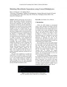
2. Mathematical modeling A fluid of viscosity µ1, injected at a uniform velocity U, displaces another fluid of viscosity µ2 (> µ1) in two-dimensional homogeneous porous media having constant permeability κ and constant porosity εp [see figure 1]. Also assume that solute dispersion in the porous medium is isotropic in nature. Fluids are considered to be miscible, incompressible, neutrally buoyant and having the same density ρ. Concentration of a solute in the solvent is denoted by c. Without loss of generality, c = 0 mol/m3 for fluid of viscosity µ1 and c = c2 mol/m3 for fluid of viscosity µ2. As the fluids are assumed miscible in nature, so a thin transition zone between the

COMSOL Multiphysics and COMSOL are either registered trademarks or trademarks of COMSOL AB. Microsoft is a registered trademark of Microsoft Corporation in the United States and/or other countries.

Excerpt from the Proceedings of the 2016 COMSOL Conference in Bangalore

fluids immediately created and we assume it has thickness δ at the beginning of our simulations, as shown in figure 1. Assume, domain of our problem is Lx x Ly and x0 is the interface position at which concentration is c = c2/2 mol/m3.

p = 0 at x = Lx ∂u = 0, v = 0 at y = 0 and y = Ly ∂x

(4) (5)

2.2 Flow in non-Darcian porous medium To describe the flow in non-Darcian porous media, various authors used a different governing equation, in place of the Darcy’s law, for conservation of momentum [3, 4, 5, 6]. Brinkman equation is an extension of Darcy's law [3] which is given by (6) ∇⋅u = 0 Figure 1: Schematic diagram of displacement of miscible fluid in 2D porous media. The dashed line shows the unperturbed fluid-fluid interface at initial time.

In the present study, the pressure gradient is the only driving force that generates the fluid flow. The complete governing system of equations are the equation of continuity [conservation of mass], the equation of motion for fluid velocity [conservation of momentum], and the convection-diffusion equation [transport of solute concentration]. The above-mentioned physical problem consists of two physics: (a) hydrodynamics, that describes the fluid motion in porous media [Darcian as well as non-Darcian porous medium]; (b) transport of solute in the porous media. Mathematical descriptions of the individual physics are described below. First, we describe the hydrodynamic part, followed by the transport of solute. 2.1 Flow in Darcian porous media Fluid motion in a porous media with lower porosity, called the Darcian porous media, is described in terms of the Darcy’s law [3, 8], (1) ∇⋅u = 0

∇p = −

µ (c) u κ

(2)

where u = (u, v), p, µ are the two-dimensional Darcy (seepage) velocity vector, hydrodynamic pressure, and the dynamics viscosity of the fluid, respectively. We assume that the dynamic viscosity of the fluid depends on a solute concentration, which is described in section 2.3 below. The boundary conditions associate with eqs. (1) and (2) are as follows, (3) u = (U, 0) at x = 0

∇p = −

µ (c ) µ (c ) 2 u+ ∇ u κ εp

(7)

Similar to the case of Darcy’s law, here also, the dynamic viscosity of the fluid depends on a solute concentration described in section 2.3 below. In this case, the no-slip boundary conditions in addition to the other boundary conditions described in eqs. (3)-(5) are required to describe the fluid motion. 2.3 Transport of solute in porous media Transport of the solute that controls the dynamic viscosity of the fluids is described by a convection-diffusion equation,

εp

∂c + u ⋅ ∇c = ε p D∇ 2 c ∂t

(8)

where D is the duffsion coeffcient. The boundary conditions associated with this equation are, c = 0 at x = 0 (9)

∂c = 0 at x = Lx ∂x ∂c = 0 at y = 0 and y = Ly ∂y

(10) (11)

Since, a transition region is of thickness δ exist between the two fluids. Hence, the initial condition for concentration [9] is given by

c(x, y, t = 0) =

" x − x0 %+ c2 ( '*1+ erf $ # δ &, 2)

(12)

where erf stands for the error function, x

erf ( x ) =

∫e

−

z2 2

dz

(13)

0

Since, an initial approximation for the fluid velocity is required to solve the convectiondiffusion equation, we presribe

Excerpt from the Proceedings of the 2016 COMSOL Conference in Bangalore

u(x, y, 0) = (U, 0)

(14) We assume an Arrheniuus type relation between viscosity and concentration [1], which is given by

µ (c) = µ1e Rc/cref

(15) where cref is the reference concentration and we can assume it, to be equal to c2 and R is the logmobility ratio and given by

!µ $ R = ln # 2 & " µ1 %

(16)

Since µ2 > µ1, so R > 0 in our problem.

3. Use of COMSOL Multiphysics® We use two different physics interfaces of COMSOL Multiphysics® to model miscible displacement in porous media. Hydrodynamic part is modeled using Darcy’s law (dl) for fluid flow in Darcian porous media, while Brinkman equation (br) is used for the non-Darcian porous media. Transport of diluted species in porous media (tds) of COMSOL multiphysics 5.2 is used to model the transport of solute concentration. These three COMSOL interfaces are described below. For our simulations, we assume glycerol as the solute and water as the solvent. Also, we consider displacing fluid is pure water. The concentration of displaced fluid (c2) is calculated from the concentrative properties of aqueous solution [10]. Parameters used in our simulations are given in Table 1.

Diffusion coefficient

D

4×10-8 m2/s

Interface position

𝑥!

0.01 m

Thickness of the transition zone

δ

10-4 m

3.1 Darcy’s law The equations used in Darcy’s law (dl) model are:

∂ (ε p ρ ) + ∇ ⋅ ( ρ u) = Qm ∂t κ u=− ∇p µ (c)

3.2 Brinkman equation The momentum conservation equations in brinkman (br) model are,

Length of domain

Lx

Value and unit 0.08 m

Width of domain

Ly

0.02 m

Log-mobility ratio

R

1, 2, 3

ρ∇ ⋅ u = Qbr

Injection Speed

U

1 mm/s

Viscosity of the displacing fluid

𝜇!

1 mPa-s

Density of both the fluids

ρ

1000 kg/m3

Porosity

εp

0.1, 0.5, 0.8

Permeability

κ

10-6 m2

Parameter

Symbol

(17b)

For constant porosity of the medium, constant density of the fluid, and zero mass source (Qm = 0), the equation of continuity, eq. (17a) reduces to the eq. (1). The inlet and outlet boundary condition specifies normal inflow velocity, U and pressure, 𝑝 = 0, respectively. No flow boundary conditions are specified at the transverse boundaries. Extra fine free triangular mesh of fluid dynamics is used for discretization of the domain. This meshing provides perturbation of triangular type at the interface.

$ ' 1 ∇ ⋅ &− pI + µ (c) (∇u + (∇u)T )) − εp &% )( * µ (c) Q ,, + β F u + br2 // u + F = 0 εp . + κ

Table 1: Lists of parameters

(17a)

(18a)

(18b)

where I is identity vector and βF is forchheimer drag coefficient. For zero mass source (Qbr = 0) the equation of continuity, eq. (18b) reduces to eq. (6). The same assumption along with zero volume force (F = 0) in the absence of forchheimer drag (βF = 0), and constant porosity reduce eq. (18a) to eq. (7). Similar to the case of Darcy’s law, the inlet and outlet boundary condition specifies normal inflow velocity, U, and pressure, 𝑝 = 0, respectively. Here, no slip boundary conditions are specified at the transverse boundaries. We use finer free triangular mesh of fluid dynamics for the domain

Excerpt from the Proceedings of the 2016 COMSOL Conference in Bangalore

discretization, which provides triangular type perturbation at the interface [see figure 2]. In the Brinkman model, the boundary layer effect are important. Hence, we also use “boundary layer” discretization of finer size near the transverse boundaries [as shown in figure 2].

transverse boundaries. Initial condition for concentration is prescribed by eq. (12). The transport of dilute species coupled with the Darcy’s law model miscible viscous fingering in Darcian porous media, while the former with the Brinkman equation model miscible viscous fingering in non-Darcian porous media.

4. Results and discussion Here we discuss the viscous instability in porous media for three porosity values, εp = 0.1, 0.5, and diffusion coefficient D used in simulations is 4x10-8 m2/s. Figure 2: Discretization of domain of finer size in Brinkman model.

3.3 Transport of dilute species in porous media Transport of diluted species in porous media (tds) model is used for the transport of solute in porous media for both the Darcy’s law and Brinkman model, since the solute transport is implicitly related to the nature of the porous media via the fluid flow equations in porous media. The equations used in ‘tds’ model are:

fingering different 0.8. The all our

4.1 Darcy’s Law Figure 3 shows the spatio-temporal evolution of the species concentration for R = 2, U = 1 mm/s. This figure depicts finger formation at the miscible interface. As time increases, coarsening of fingers, and hence the reduction in number of fingers are observed. Shielding of adjacent finger reduces the supply of less viscous fluid and results fading of advanced fingers.

∂ci + P2,i + ∇ ⋅ Γ i +u ⋅ ∇ci = Ri + Si (19a) ∂t P1,i = ε p (19b)

P1,i

∂ε p ∂t N i = Γ i +uci = −De,i ∇ci + uci

P2,i = ci

De,i =

εp DF,i τ F,i

(19c) (19d) (19e)

where ci, Γi, Ri, Si, De,i, DF,i and 𝜏!,! are the concentration, diffusive flux, reaction rate, source, effective diffusion, molecular diffusion and tortuosity of the i-th species [i = 1, 2], respectively. We use tortuosity model which gives, 𝜏!,! = 1. Now for constant porosity and constant diffusion, 𝑃!,! = 0 and ∇ ⋅ Γ! = ∇ ⋅ −𝜀! 𝐷!,! ∇𝑐! = −𝜀! 𝐷!,! ∇! 𝑐! . Thus, the system of eqs. (19a)–(19e) reduce to the convectiondiffusion eq. (8) for constant porosity, constant diffusion, Ri = 0, Si = 0 and 𝜏!,! = 1. The inlet boundary condition specifies species concentration, c = 0 and outlet boundary condition is corresponds to free flow. No flux boundary conditions are specified at the

Figure 3: Spatio-temporal evolution of the species concentration at time t = 0, 5 and 10 seconds [from top to bottom] for R = 2 and U = 1 mm/s.

It is observed that the instability increases with R [see Figure 4]. Figure 5 depicts the splitting of fingers for R = 3. This figure depicts that the tip of the finger widen before it splits into two fingers. These summarize that our present

Excerpt from the Proceedings of the 2016 COMSOL Conference in Bangalore

COMSOL model successfully capture miscible VF in homogeneous porous media along with various nonlinear aspects of miscible VF [1].

Next, we discuss the effect of porosity on the observed VF patterns. Figure 6 depicts that the fingering dynamics are different for εp = 0.1 and εp = 0.5 at time t = 2 and 10 seconds, respectively. In both the cases, characteristics time ‘t/εp’ is same. But in the later case, spreading of advanced fingers is less and also reduction in number of fingers are observed. This is due to more stabilizing effect of diffusion [11] in the latter case. 4.2 Brinkman equation

Figure 4: Spatio-temporal evolution of the species concentration at time t = 5 seconds for R = 1 [top], 3 [bottom], U = 1 mm/s.

For εp = 0.8, i.e. for the Brinkman equation, the fingering dynamics are significantly different from that with Darcy’s law. Figure 7 shows the snapshots of the species concentration at different times for R = 3, U = 1 mm/s. Comparing this figure with figure 5 [corresponding to the Darcy’s law], we observe that the fingering instability is prominent with the Darcy’s law compared to the Brinkman model. In the later case, boundary layer formation is observed, which is absent in Darcy’s law model. Also, we observe that the instability sets in very late in the later case compared to the former. The wavelength of the unstable modes is large by a factor of 4 in the Brinkman model in comparison to the Darcy’s law. We further observe that for R = 1 no fingering is observed. Here, also it is observed that the instability increases with R same as Darcy’s law [see Figure 8].

Figure 5: Spatio-temporal evolution of the species concentration at time t = 5 seconds [top], 6 seconds [bottom] for R = 3, U = 1 mm/s.

Figure 6: Spatio-temporal evolution of the species concentration for εp = 0.1 at t = 2 seconds [top] and εp = 0.5 at t = 10 seconds [bottom], where R = 2, U = 1 mm/s.

Figure 7: Spatio-temporal evolution of the species concentration at time t = 10, 20, 30 seconds [from top to bottom] where R = 3, εp = 0.8, U = 1 mm/s.

Excerpt from the Proceedings of the 2016 COMSOL Conference in Bangalore

media with inertia effects is the focus of our ongoing research.

6. References

Figure 8: Spatio-temporal evolution of the species concentration for R =1 [top], 3 [bottom] at t = 30 seconds, where εp = 0.8, U = 1 mm/s.

Near the transverse boundaries, similar fingering patterns are observed for given set of parameters in Darcian as well as non-Darcian porous media. This is due to similar perturbation near the transverse boundaries. In our model, perturbations at the interface are inserted by triangular mesh only. Finite element simulations of our problem are sensitive to the type and refinement of the mesh used. When mapped meshing is used for discretization of the domain, only diffusion at the interface is observed. Since mapped mesh is structured meshing, there is no perturbation at the interface. Nevertheless, fingering instability is observed by modifying the initial condition for the COMSOL simulations when we introduce a random perturbation at the interface by adding a solid line for ensuring nodes at this interface.

5. Conclusions

[1] G. M. Homsy, Viscous fingering in porous media, Annu. Rev. Fluid Mech., 19, 271-311 (1987) [2] S. Pramanik, G.L. Kulukuru, and M. Mishra, Miscible viscous fingering: Application in chromatographic columns and aquifers, COMSOL conference, Bangalore (2012) [3] D. A. Neild, and A. Bejan, Convection in porous media, 5-14, Springer-Verlag, Berlin (1992) [4] L. Durlofsky, and J. F. Brady, Analysis of the Brinkman equation as a model for flow in porous media, Phys. Fluids, 30(11), 3329-3341 (1987) [5] R. Booth, Miscible Flow Through Porous Media, University of oxford (Ph.D. thesis) (2008) [6] P. Forchheimer, Wasserbewegung durch Boden, Zeit. Ver. Deutscher. Ing., 45, 1781-1788 (1901) [7] E. Holzbecher, Modeling of viscous fingering, COMSOL conference, Milan (2009) [8] H. Darcy, Les Fontaines Publiques de la Ville de Dijon. Dalmont, Paris (1856) [9] N. Goyal, and E. Meiburg, Miscible displacement in Hele-Shaw cells: twodimensional base states and their linear stability, J. Fluid Mech., 558, 329-355 (2006) [10] A. V. Wolf, Aqueous Solutions and Body Fluids, Hoeber Medical Division, Harper & Row, New York (1966) [11] S. Pramanik, and M. Mishra, Effect of Péclet number on miscible rectilinear displacement in Hele-Shaw cell, Phys. Rev. E, 91, 033006 (2015)

We present a new numerical model of COMSOL Multiphysics by coupling of two different physics to capture miscible viscous fingering in two-dimensional homogeneous porous media with small as well as large porosity. We successfully capture the nonlinearities of miscible VF, such as shielding, spreading, and splitting, with the help of Darcy’s law. This is in accordance with the results of the existing literature [1]. The effects of various flow parameters on the observed viscous fingering are discussed. For porous media with large porosity Brinkman equation shows different instability dynamics both qualitative and quantitatively. Modeling miscible viscous fingering in porous

Excerpt from the Proceedings of the 2016 COMSOL Conference in Bangalore