concept formation in dimensional spaces - Lund University Cognitive

CONCEPT FORMATION IN DIMENSIONAL SPACES Peter Gärdenfors and Kenneth Holmqvist L u n d U n i v e r s i ty C o g n i ti v e S c i e n c e Kungshuset, Lundagård S–223 50 Lund, Sweden E-mail: [email protected], [email protected]

1. INTRODUCTION This article presents a series of experiments on concept formation. These experiments compared four different categorisation rules. The rules presume that the stimuli to be classified can be modelled psychologically as points in a dimensional space (Shepard 1987, Gärdenfors 1990a, 1990b). Two of the rules are based on the assumption that there are prototypical representatives of a concept, a third rule is a “nearest neighbour” model, and the fourth is based on average distances (Reed 1972), where distances are measured in the dimensional space. Before giving a more precise description of the categorisation rules and the experiments, we will present the general theoretical approach that is adopted.

1.1 Theoretical background In this article, we take c a t e g o r i s a t i o n to be a rule for classifying objects. The result of categorisation will be a number of c o n c e p t s . The concepts will generate classifications of stimuli. In the model presented here, where stimuli are represented as points in dimensional spaces, a categorisation will generate a partitioning of the space and a concept will correspond to a region of the space. One can find many proposals for categorisation rules in the philosophical and psychological literature. A classical example is Aristotle’s theory of necessary and sufficient conditions (see Smith and Medin (1981) for a presentation of this and other theories of concept formation). His view on how concepts are determined has had an enormous influence throughout the history of philosophy. As is shown by numerous experiments (e.g. Rosch 1975,

1978, Labov 1973, Mervis and Rosch 1981, Smith and Medin 1981), the Aristotelian theory is not realistic as a cognitive or psychological account of how people form and use concepts. As a result of a growing dissatisfaction with the classical theory of concepts, several alternative theories have been developed within cognitive psychology. The most well known is p r o t o t y p e theory (e.g. Rosch 1975, 1978, Mervis and Rosch 1981, Lakoff 1987). The main idea of this theory is that within the class of objects falling under a concept certain members are judged to be more representative of the concept than others. The most representative exemplars of a concept are called p r o to ty p i c a l members. A given set of prototypes for a class of concepts can be used for generating a categorisation by the rule that a stimulus is classified according to which prototype it is most similar to. However, even if prototype theory fares much better than the Aristotelian theory in explaining how people use concepts, the theory does not explain how such prototype effects can arise as a result of learning to use our concepts. The theory can neither account for how new concepts can be created from relevant exemplars, nor explain how the extensions of concepts are changed as new concepts in the same category are learned. The purpose of this article is to present four models based on a “dimensional” or “geometric” approach to categorisation, together with the experiments that we have performed in order to test the models. The key notion is that of a conceptual space consisting of a number of dimensions which are used as the framework for various categorisation rules. A conceptual space can be seen as a geometric structure for which several categorisation rules can be formulated and tested. We want to show that a model based on conceptual spaces together with a classification rule based on so called Voronoi

Lund University Cognitive Studies – LUCS 26 1994. ISSN 1101–8453.

tioning and extinction. Needed as they are for all learning, these distinctive spacings cannot themselves all be learned; some must be innate.

tessellations can provide us with an explanation of how concepts are formed and develop, at least for certain classes of objects. The space used in our experiments is a representation of shell shapes.

Let us now turn to an outline of how conceptual spaces may be used as a basis for a theory of categorisation. A first rough idea is to describe a concept as determined by a r e g i o n of a conceptual space S, where “region” should be understood as a spatial notion determined by the topology and metric of S. For example, the point in the time dimension representing “now” divides this dimension, and thus the space of vectors, into two regions corresponding to the concepts “past” and “future”.

There are several related studies in the psychological literature. Reed’s (1972) investigation of classifications of Brunswick faces uses an approach that is similar to ours, even if the “space” of faces has a very limited structure in comparison to the shell space presented below. Similarly, Ashby and Gott’s (1988) investigations of decision rules for categorising multidimensional stimuli are based on a methodology that shares many features with ours. Some further examples of studies of concept formation that utilise dimensional notions are Pittenger and Shaw (1975) on faces, Labov (1973) on cups, Nosofsky (1986) on semicircles, and Nosofsky (1988) on colours.

Shepard (1987, p. 1319) gives an evolutionary argument that supports this proposal: An object that is significant for an individual’s survival and reproduction is never sui generis; it is always a member of a particular class – what philosophers term a “natural kind.” Such a class corresponds to some region in the individual’s psychological space, which I call a consequential region. I suggest that the psycho-physical function that maps physical parameter space into a species’ psychological space has been shaped over evolutionary history so that consequential regions for that species, although variously shaped, are not consistently elongated or flattened in particular directions.

1.2 Conceptual spaces and the geometric categorisation models In this subsection, we introduce the notion of a c o n ceptual space which serves as a theoretical framework for the different categorisation models. A conceptual space consists of a number of quality dimensions. The dimensions that will be considered in this article are assumed to be generated by our perceptual mechanisms, but in a general theoretical investigation one may consider quality dimensions that are of a more abstract non-sensory character. As examples of quality dimensions one can mention colour, pitch, temperature, weight, and the three ordinary spatial dimensions.

One way of giving Shepard’s idea a mathematical formulation is the following criterion where the topological characteristics of the quality dimensions are utilised to introduce a spatial structure on categories (cf. Gärdenfors 1990a, 1990b):

The notion of a dimen sion should be understood literally. It is assumed that each of the quality dimensions is endowed with a certain topological or metric structure. This structure can be determined by psycho-physical investigations. For example, perception of weight is one-dimensional with a zero point, isomorphic to the half-line of non-negative numbers; and the hue of a colour can be represented by a circular dimension (see e.g. Gärdenfors 1990a, 1992).

C r i t e r i o n P : A n a t u r a l c a t e g o r y is a convex region of a conceptual space. A c o n v e x region is characterised by the criterion that for every pair of points v 1 and v 2 in the region all points b e t w ee n v 1 and v 2 are also in the region. The motivation for the criterion is that if some objects are located at v1 and v2 in relation to some quality dimension (or several dimensions) and both are examples of the category P, then any object located between v1 and v2 on the quality dimension(s) will also be an example of P. Criterion P presumes that the notion of “betweenness” is meaningful for the relevant quality dimensions. This is, however, a rather weak assumption that demands very little of the underlying topological structure. However, in what follows we shall work with the stronger assumption that the dimensions we consider have a metric so that we can also talk about distances between points in the space.

We cannot provide a complete list of the quality dimensions generated by our perceptual mechanisms. Some of the dimensions seem to be innate and to some extent hardwired in our nervous system, as for example colour, pitch, and probably also ordinary space. Other dimensions are presumably learned. Learning new concepts often involves expanding one’s conceptual space with new quality dimensions. Quine (1969:123) notes that something like a conceptual space is needed to make learning possible: Without some such prior spacing of qualities, we could never acquire a habit; all stimuli would be equally alike and equally different. These spacings of qualities, on the part of men and other animals, can be explored and mapped in the laboratory by experiments in condi-

In support of Criterion P it can be shown that if prototype theory is combined with the idea of a metric conceptual space as a framework for categorisation, then

2

the representation of categories as convex regions is to be expected. To see this, assume that some quality dimensions of a conceptual space are given, for example the dimensions of colour space, and that we want to partition it into a number of categories, for example colour categories. If we start from a set of prototypes p 1 , ..., p n of the categories, for example the focal colours, then these should be the central points in the categories they represent. One way of using this information is to assume that for every point p in the space one can measure the distance from p to each of the pi’s. If we now stipulate that p belongs to the same category as the closest prototype pi, it can be shown that this rule will generate a partitioning of the space that consists of convex areas (convexity is here defined in terms of the assumed distance measure). This is the so called Voronoi tessellation, a two-dimensional example of which is illustrated in Figure 1.

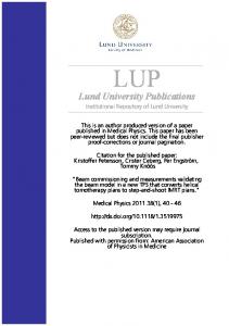
Furthermore, when the subject sees a new item in a category, the prototype for that category will, in general, change somewhat, since the mean of the class of examples will normally change. Figure 3 shows how this categorisation is changed by the addition of one new exemplar, marked by an arrow, to one of the categories. This addition shifts the prototype of that category, which is defined as the mean of the exemplars, and consequently the Voronoi tessellation is changed. The old tessellation is marked by hatched lines.

p3

p2 p

Figure 2. Voronoi tessellation generated by three clas ses of exemplars.

1 p4 p6 p

new

5

Figure 1. An example of a Voronoi tessellation of the plane into convex sets determined by a set of prototypical points.

Thus, assuming that a metric is defined on the subspace that is subject to categorisation, a set of prototypes will, by this method, generate a unique partitioning of the subspace into convex regions. Hence there is an intimate link between prototype theory and the analysis of this article where categories are described as convex regions in a conceptual space. Figure 3. Change of Voronoi tessellation in Figure 2 after adding a new exemplar.

In the experimental investigations, we assume that the prototype for a category is determined from the set of exemplars of the category that a subject has seen. The rule we employ for calculating the prototype from a class of exemplars is that the ith coordinate pi for the vector representing the prototype is the mean of the ith co-ordinate for all the exemplars. Applying this rule means that a prototype is not assumed to be given a priori in any way, but is completely determined by the experience of the subject. Figure 2 shows how a set of 9 exemplars, represented as differently filled circles, grouped into three categories generate three prototypical points, represented as black crosses, in the space. These prototypes then generate a Voronoi tessellation of the space.

The Voronoi tessellation generated from a set p1, ..., pn of prototypes yields the following decision rule for categorisation:1

Prototype Voronoi categorisation (PV): An object represented as a vector xi in a conceptual space belongs to the

category for which the corresponding prototype is the closest, i.e., the pj that minimises the distance between xi and pj. A drawback of the standard Voronoi tessellation is that 1 This rule is the same as the “Prototype model” in Reed (1972).

3

it is only the prototype that determines the partitioning of the conceptual space. However, it is quite clear that for many natural categorising systems some concepts correspond to “larger” regions than others. For example, the concept “duck” covers a much larger variety of birds than “ostrich,” even though both concepts are basic level concepts in the terminology of Rosch (1978), i.e., they are both members of the same categorisation of birds.

cv

V

W cw

So the question arises whether there is some way of generalising the Voronoi tessellation that can account for varying sizes of concepts in a categorisation, but which will still result in a convex partitioning of the underlying conceptual space. It can be shown (see Holmqvist and Gärdenfors, in preparation) that such a generalisation is possible. The standard Voronoi tessellation is based on the ordinary Euclidean metric, so that in order to determine the lines that form the tessellation one solves the equation

cu

U

Figure 4. An example of a generalised Voronoi tessellation determined by the circles. The generalised Voronoi tessellation is represented by continuous lines and the prototype Voronoi tessellation by dashed lines.

Before the generalised Voronoi tessellation can be applied, the values cv must be determined. A natural choice, that we will use throughout this article, is to define cv as the magnitude of the s t a n d a r d d e v ia t i o n of the exemplars from the prototype. This choice entails that the generalised Voronoi tessellation can be completely determined from the co-ordinates of the exemplars of the different categories.

!i (vi – xi )2 = !i (wi – xi )2 where v = (v1 ,...,vn) and w = (w1 ,...,wn) are the vectors of two prototypical points in the conceptual space. However, instead of saying that there is only a prototypical point for a particular concept one can introduce the notion of a prototypical area and then determine a gen er a l i s e d Voronoi tessellation by computing distances from such areas instead. In relation to the earlier example, the prototypical area for ducks could then be taken to be larger than the corresponding area for ostriches. We model this idea by assuming that the prototypical area for a concept can be described by a circle with centre (v1 ,...,vn) and radius cv . By varying the radius, one can change the size of the prototypical area (for example, the cv for ducks would be larger than that for ostriches).

The generalised Voronoi tessellation corresponds to the following rule for categorisation:

Gen er alised Vor on oi categor isation (GV): An object represented as a vector xi in a conceptual space belongs to the category for which the corresponding prototypical circle is the closest. Following Reed (1972), we will compare the results of the two Voronoi rules PV and GV to two other categorisation rules:

In order to determine the generalised Voronoi tessellation one then solves equations of the form

Nearest neighbour categorisation (NN): An object represented as a vector xi in a conceptual space belongs to the category to which the exemplar that is closest to x i is included.2

!i (vi – xi )2 – cv = !i (wi – xi )2 – cw It can be proven (Holmqvist and Gärdenfors, in preparation) that for all choices of prototypical circles, this equation generates a set of straight lines that will partition the space into convex subsets. A simple illustration of a generalised Voronoi tessellation is given in Figure 4. The prototype Voronoi tessellation generated from the centres of the circles, corresponding to the prototypes, is indicated by hatched lines.

Average distance categorisation (AD): An object represented as a vector xi in a conceptual space belongs to the category to which xi has the smallest average distance to the examples for the category. The four rules that have been introduced here often result in very similar categorisations. As a consequence, it will become difficult to distinguish between them in empirical tests of which rule best describes the behavior of subjects in classification tasks. Figure 5 illustrates an extreme case where the four rules generate clearly separate partitionings.

The metric generated by this kind of equation will not be Euclidean. All points on the prototypical circle will have distance zero from the prototype, and it turns out that points within the circle will have imaginary numbers as distances.

2 Reed (1972), pp. 385-86, calls this rule the “proximity algorithm”.

4

GV

PV

AD

AD

NN

NN

Figure 5. An example of how the four categorisation rules result in extremely different categorisations of the space. The two filled dots are exemplars of one category and the cross between them its prototype. The unfilled dots are exemplars of another category, again with its prototype marked as a cross between them. PV, GV, NN and AD denote partitionings generated by the four categorisation rules.

pictures as shells, they normally have no “prejudices” concerning how shells are actually classified in biology. This means that we can “create” new categories for the subjects by showing appropriate shells, i.e., more or less prototypical examples, in a desired region of the shell space.

1.3 The shell space In order to evaluate the four models presented above we have performed a series of experiments concerning the categorisation of shell shapes. There are several reasons why shells constitute a useful domain for empirical investigations:

2. PILOT STUDIES

(1) It is possible to generate a great number of fairly realistic shell shapes in a conceptual space that is built up from three dimensions. (This space will be described below.)

In order to obtain an estimate of the metric space underlying perceptions of shell forms, we performed three pilot studies. These studies can be seen as calibration experiments determining the scaling solution of the underlying dimensions. The results of the experiments strongly confirm the hypothesis that the psychophysical shell space is indeed three-dimensional with an identifiable metric. The perceptually grounded metric that was estimated during the pilot studies is the one that was used in the two main experiments where the four categorisation rules presented above are evaluated. It is also the metric used below in Figures 8 and 11 where we illustrate the various classification tasks.3

(2) The shells can easily be drawn by a graphic program where the only inputs are three co-ordinates in the shell space. (3) The pictures generated by our program are identified by the subjects as pictures of realistic 3D shells. They are thus much more natural than most of the stimuli used in classification tasks in current cognitive psychology, like e.g. the dot-patterns (Posner and Keele 1968, Shin and Nosofsky 1992) or the semi-circles with an additional radius (Nosofsky 1986, Ashby and Lee 1991). Not even the schematic faces used by Reed (1972) have a very high degree of “ecological validity” (Gibson 1979).

3 The metric is not identical to the one used in the graphics program but a simple transformation of it.

(4) Even though test subjects recognise the object on the

5

2.1 Stimuli

spiralling way. The shape of the shell is, according to Raup (1966), largely determined by three factors (see Figure 6):

Throughout all experiments, we used depictions of shell shapes as stimuli. A shell normally grows in a

Coiling axis

Initial generating curve

V

R

E

Generating curve after one generation

Figure 6. The three dimensions V, E, and R, generating a shell shape.

are generated by our graphics program. The only input to the program are the three co-ordinates.

(1) The rate E of whorl expansion which determines the curvature of the shell. The rate E is assumed to be a constant defined as the quotient en+1 /en between the distance en+1 of the central point to the generating axis and the distance en one revolution earlier. Small curvature results in densely spiralled shells, while a high curvature produces openly spiralled shapes.

The three dimensions V, E, and R, span a space of possible shell shapes that is suitable for testing the four models of categorisation described above. However, the dimensional space is defined with the aid of three mathematical dimensions. As a preliminary step, it is necessary to test the psychological validity of the hypothesis that our perceptions of shells also form a three-dimensional space. But even if the perceptual shell space is three dimensional, it does not at all follow that the metric of the space is the same as the mathematical co-ordinates used by the graphic program.4 Before we can apply the four categorisation

(2) The rate V of vertical translation along the coiling axis. The rate V is also assumed to be a constant. It is defined as the quotient vn+1 /v n between the vertical distance vn+1 of the central point to the initial level on the generating axis and the corresponding distance vn one revolution earlier. Having no vertical translation yields flat shells, while rapid growth results in elongated shapes.

4 It seems to us that this point is sometimes missed in the psychological literature. For example Ashby and Gott (1988) work with stimuli composed of two lines, one horizontal and one vertical, joined at the upper left corner (cf. their figure 2 on p. 35). The stimuli are described by a two dimensional vector (x,y) where x denotes the length of the horizontal component and y the length of the vertical component. Throughout the article, Ashby and Gott discuss the space generated by these axes and define their decision rules using this metric. However, from a number of observations in their article which are problematic for them, it seems that these co-ordinates do not produce an appropriate metric for the perceptual space producing the categorisations. It seems to us that if one makes a co-ordinate shift by defining x' = x/y and y' = x "y, one obtains a metric that is much better suited to explain the observed phenomena. The dimension x' measures the proportions of the lengths of the two line segments, while y' is a measure of the relative size of the stimulus.

(3) The expansion rate R of the generating curve (the aperture) of the shell. Our graphic program only operates with a circular generating curve, but one finds in nature a large variation of the outline of the apertures (which is largely determined by the shapes of the soft body of the molluscs). The growth rate R, which is assumed to be constant, is defined as the quotient rn+1/rn between the radius rn+1 and the radius rn one revolution earlier. Slow growth results in tube formed shells. Very rapid growth produces shells that look like in Figure 7c below. Figure 7 shows some examples of shapes that are produced by different combinations of values for the coordinates. All shell pictures here and in the following

6

models it is necessary to establish the relevant psychological metric, i.e., the scaling solution, of the shell

space.

Figure 7. Some examples of shell shapes drawn by the graphic program together with their generating co-ordinates (rate of whorl expansion, vertical growth, growth of radius of aperture).

This methodology is completely in line with Shepard’s (1987, p. 1318) recommendations for how psychological laws should be obtained:

a psychological space might attain invariance.

2.2 Calibration of Stimuli

Analogously in psychology, a law that is invariant across perceptual dimensions, modalities, individuals, and species may be attained only by formulating the law with respect to the appropriate abstract psychological space. The previously troublesome variations in the gradient of generalisation might then be attributable to variations in the psycho-physical function that, for each individual, maps physical parameter space (the space whose co-ordinates include the physical intensity, frequency, and orientation of each stimulus) into that individual’s psychological space. If so, a purely psychological function relating generalisations to distance in such

The three dimensions given by Raup’s (1966) model are not the most natural ones from a perceptual point of view. When estimating the vertical and horizontal growth rates of shells, we don’t look at the centre of the generating circle. Instead we focus on its extreme points in the vertical and horizontal direction, loosely speaking the height and width of the shell. This means that the vertical and horizontal expansion rates should instead be described by the following values: V' = V + R – 1 E' = E + R – 1

7

This shift of co-ordinates will not change the distances between the points in the space. Using the space generated by the dimensions V', E', and R, we wanted to check whether further transformations of the dimensions were necessary to obtain a satisfactory description of subjects’ perceptions of shell forms. The transformations we tested for each of the dimensions were instances of Stevens’ power law d'(x) = k(d(x))b.5 Since there were three dimensions (V', E' and R), we should estimate the values of six parameters kV' , kE' , kR and bV' , bE', bR.

used were drawn from a large number of points that we picked out from all over the shell space. In both the similarity and the classification questions, subjects were asked to indicate the similarities on a continuous scale. Subjects were tested singly. Before starting, the subject was given instructions about the tasks. The shells were then presented on ordinary sheets of paper. First we presented the 25 similarity questions and then the 14 classification questions, both in a random order. We did not put any time limits on the subjects, nor did we measure the time it took them to complete the test.

2.3 Pilot study 1 Method, design and procedure

Subjects

In the pilot studies, subjects were given two types of questions :

Thirteen subjects (colleagues and friends) participated in this first pilot study. They were not paid for participation.

(i) Similarity judgements

Response coding

Subjects were presented with three shell drawings (produced by our program) on a sheet of A4 paper. Each shell was presented from two views, one side and one top view. Subjects were asked to judge whether the shell in the middle was more similar to the shell to the left than to the one to the right.

Answers to similarity questions were interpreted in the following way: Assume that a subject placed the X representing the middle shell 3 cm from the endpoint representing the left shell. We then let the middle of the scale be 0, with endpoints –10 and 10, and this distance answer be coded as –7. With this encoding, we calculated the average for each similarity question of test sheet distances over test subjects.

Subjects answered these questions by putting an X on a 20 cm long line along the bottom of the paper. The endpoints of the line represented the two outer shells, while the line indicated the perceived perceptual distance between those two shells. The X drawn by a subject was to mark the perceptual position of the middle shell in relation to the two outer shells.

The hypothesis was that this average of the distances on the test sheet should correlate with the corresponding distances in the shell space. We therefore calculated the distance dleft in the shell space between the middle and left shells and the distance dright between the middle shell and the right shell. The distance value in the shell space was then calculated as dleft – dright . This averaged test sheet distances for the similarity questions was then correlated against corresponding shell space distances6 .

(ii) Classification judgements In addition to the similarity questions, subjects were also asked to provide classification judgements. Subjects first saw two groups of pictures of exemplars of shells (three or four shells in each group). They were then shown a picture of a new shell and asked to classify this shell into one of the two groups. In pilot study 1, each classification question involved two groups of exemplars, drawn from a total of four groups of exemplars.

Answers to classification questions were analysed in the same way, with one exception. In classification questions, we did not have single left and right shells but instead a group of exemplar shells for the left and right categories. Therefore, when we used the four models PV, GV, NN and AD to calculate the distances from the middle shell to each of the two categories in the shell space. These two distances could then be used to calculate the proportion value that we needed.

The classification judgements serve as tests of the predictions of the different categorisation rules discussed above. These tests will be the focus of the two main experiments described in Sections 3 and 4.

It should be noticed that the distances depend on the metric chosen. In our case the metric varied with the values of the vector (kV' , kE', kR, bV' , bE', bR) of constants for the three instances of Stevens’ power law that were used. As we correlated the proportion values we also varied the vector so as to maximise the correlation

All subjects received 25 different similarity questions and 14 classification questions. All shell forms that we 5 An alternative method would have been to use multi dimensional scaling (Shephard 1962a,b, 1987). However, this would have involved asking the subjects to make comparisons of the relative similarity of pairs of shell figures, instead of the question concerning triples of shells that was used in our pilot studies.

6 Throughout all experiments, we used the standard Pearson r-correlation.

8

coefficient. This was our way of estimating the calibration of the stimuli (as we noted above), which was necessary for the correct calculation of distances as we compared the four categorisation models.

basis of the results of the first study, would be as informative as possible. The different pairs of shells were distributed over the entire shell space and along all three dimensions, but also diagonally through the space. We used 14 different similarity questions. No classification questions were asked.

Results Using the space generated by the dimensions V', E' and R, with the non-transforming power vector (1,1,1,1,1,1), we obtained a correlation coefficient of 0.70. However, by replacing these dimensions with the transformations generated by varying the b-coefficients only, the correlation could be improved considerably so that the vector (1, 1, 1, 0.88, 1, 0.58) yielded a correlation of 0.86. The three b-coefficients confirmed our intuitions about the relative prominence of the three dimensions.

The shells were again presented on ordinary A4 sheets of paper, but this time each shell was presented only from the side view as in Figure 8. The other difference from pilot study 1 was that in this study, subjects were asked to indicate the similarities in a 3-alternative forced choice response as in Figure 8. Subjects Ten people, consisting of a mixture of colleagues and computer science students, mostly male, served as subjects. None was paid for their participation.

At this early stage, we performed only a preliminary analysis of the answers to classification questions made by the subjects. The results suggest that Nearest neighbour categorisation (NN) and Generalised Voronoi categorisation (GV) produced better predictions than Prototype Voronoi categorisation (PV) and Average distance categorisation (AD): Out of the fourteen classification questions, NN predicted eight of the modal answers among subjects and GV predicted seven clear cases and three borderline cases (where there was no clear modal response).

Response coding In calculating the results, we basically used the same correlation between averaged test sheet distances and shell space distances as in pilot study 1. The difference was that in this study, answers were discrete. We therefore had to replace the average test sheet distances with an average of the subjects’ 3-alternative answers, each of which was coded as –1, 0 and 1.

Discussion

Results

We learned from this pilot study that the top view of the shells did not contribute much information about the shell shapes. Since they also made the interpretation of shapes more difficult because the subjects had to integrate two pictures of a shell to make a judgement, we decided to only use the side view of the shell in the following studies.

As a consequence of aiming at making the similarity judgements as informative as possible about the psychophysical constants, we only obtained a correlation of 0.30 using the space generated by the dimensions V', E' and R, without any transformation. However, the transformations of this space generated by the optimal vector (1, 1.55, 1, 1.72, 1, 0.99) gave a correlation as high as 0.92.

Furthermore, letting subjects mark their answers on a continuos scale gave less information than we had hoped for. The subjects tended to cluster their answers around three or four points along the scale, thus making it tantamount to a discrete set of answer options. We therefore replaced the continuos line with discrete alternatives in the following studies.

Discussion The result strongly confirms our hypothesis that it is possible to identify an underlying perceptual shell space of shell forms with sufficient accuracy. Since small changes of the optimal vector resulted in clearly smaller correlation coefficients, we decided to use the calibrated shell space generated by this vector in the main experiments.

2.4 Pilot study 2 Method, design and procedure

Pilot study 2 revealed the calibration of the three dimensions V', E' and R, but it was still not certain that the dimensions are orthogonal. This would be tested in pilot study 3.

The motivation for the second study was to make a more precise determination of the vector of constants in the three power laws. To this end, we aimed at choosing examples of similarity judgements that, on the

9

Figure 8. Example of judgements of similarities. Subjects were asked to check one of the squares.

2.5 Pilot study 3

they give linearly independent contributions to the perceptions of shell forms. This means that each of the dimensions can be modified independently of the others. The operationalisation of the orthogonality test can best be explained with the aid of Figure 9.

In order to further establish the validity of the perceptual shell space that has been identified, we wanted to check whether the dimensions V', E' and R are orthogonal to one another. If the dimensions are orthogonal,

y

(x0, y1)

y

(x0, y1)

d1 d1

(x0, y0)

d2

(x1, y0)

(x0, y0)

x

d2

(x1, y0)

x

Figure 9. Operational test of orthogonality.

10

To show that the axes x and y (with a given metric) are orthogonal to one another, subjects are asked to compare the similarity of an object with co-ordinates (x0 , y1 ) to objects with co-ordinates (x0 , y0 ) and (x1 , y0 ) where x1 is relatively close to x0 . If the axes are orthogonal as in the left part of Figure 9, then (x0 , y1 ) should be judged to be more similar to (x0, y0 ) than to (x1 , y0 ) since d1 is smaller than d2 . However, if the axes are not orthogonal as in the right part of the figure, this may not hold since the distance d2 between (x0 , y1 ) and (x1 , y0 ) may then be smaller than the distance d1 between (x0 , y1 ) and (x0 , y0 ).

2.6 General Discussion The data obtained from the three pilot studies suggest that we have identified a psychological space for similarity judgements of shell shapes. The orthogonality of the dimensions in this space is reasonably supported and the metric of the space is sufficiently well identified. On the basis of the results obtained, we felt confident in proceeding to the main classification experiments. One complication should be mentioned, though. During the pilot tests (as well as during the main experiments) we took notes of the spontaneous comments from the subjects after they had finished the similarity judgements. One frequent comment was that when judging the similarity of different shells, or when classifying them, they looked for whether the shell was “closed” or “open” in the sense that a shell was “closed” if the aperture overlaps with the previous whorl of the shell (cf. the A-shells in Figure 12) and “open” if it was separated from it (cf. the B-shells in Figure 12). This gestalt feature7 of the shells was added as a fourth dimension in the power law analysis in pilot study 1. The resulting vector is (1, 1, 1, 0.90, 1, 0.60, 0.015, 0.68), where the two last numbers are the k- and bparameters of the “openness” dimension. This resulted in a correlation coefficient of 0.862 which is almost identical with the correlation obtained without the openness dimension. Furthermore, the values for the other dimensions were very close to the previous values where the openness dimension was not included. Consequently, we did not include this factor in our subsequent analysis.

Method, design and procedure In this pilot study, we used 24 different similarity judgement questions but no classification questions. The similarity questions were all of the form indicated in Figure 9, but the metric of the two axes were given by the dimensions V', E' and R. We used the same procedure as in pilot study 2. The shells were presented on ordinary A4 sheets of paper, and each shell was presented only from the side view, as in Figure 8. Also in this study, subjects were asked to indicate the similarities using a 3-alternative forced choice. Subjects The subjects were 10 computer science students, all male, between ages 20 and 28. Again, no one was paid for participation, nor did we put any time limits or measure the time subjects used. Response coding The analysis in pilot study 3 was identical to the analysis made in pilot study 2.

3. EXPERIMENT 1 The goal of the two main experiments was to evaluate the four classification rules that were presented in section 1.2, i.e., Nearest Neighbour categorisation (NN), Generalised Voronoi categorisation (GV), Prototype Voronoi categorisation (PV), and Average Distance categorisation (AD). The preliminary results from pilot study 1 suggest that the best predictors are NN and GV.

Results Using the uncalibrated space generated from V', E' and R, we obtained a correlation coefficient of 0.72 between the subjects answers and the distances in that space. However, we had not calibrated the similarity questions in the test with respect to the vector that was estimated in pilot study 2. This defect may explain the comparatively low correlation. By investigating the power law transformations of this space, we found that the vector (1, 1.35, 1, 1.5, 1, 1) gave a maximum correlation of 0.80.

The two main categorisation experiments were based on different set-ups. In the first experiment (to be described in this section), all the exemplars that were used to induce a category for a subject were visible on sheets of papers during the classifications of new test shells, so that exemplars and test shell could be directly compared. We later assumed that such a set-up would favour the NN model, which functions by comparing test shells to the exemplars. In contrast, the second experi-

Discussion Even if this result is not identical with the results in pilot study 2, the general pattern of parameters is the same. This result suggests that the dimensions, with the metrics estimated in pilot study 2, have a sufficient degree of orthogonality to be treated as independent perceptual dimensions.

7 We call it a gestalt feature, because the values for the three generating dimensions determine whether the shell is ”closed” or ”open”.

11

ment (described in Section 4), required subjects to learn the category from the exemplars which were presented on a computer screen. These exemplars were not shown when the new shells to be classified were presented.

the different models are in general very close to one another. Consequently, the difference between the predicted response frequencies are not very large. Furthermore, the points in the psychological space where the models yield different predictions sometimes correspond to comparatively unnatural shells. A consequence of this is that the stimuli are difficult to classify for the test subjects. Hence we did not expect any accuracy in the predictions of the models, only that the relative differences would be so large that we could distinguish between the models.

We expected that the closer a shell lies to a border between two categories in the psychological space the more diversity we will find in the classification answers from the subjects. In order to model this intuition, we defined, for each of the four categorisation models, a predicted response frequency for a given category x. Each of the four models provides a distance measure that determines the distance from the stimulus shell x to any category n. For PV, dPV (x,n) is the distance between x and the prototype for category n. For GV, dGV (x,n) is the distance between x and the prototypical circle for category n.8 For NN dNN (x,n) is the distance between x and the nearest shell in category n. For AD, finally, dA D (x,n) is the average distance between x and the instances of category n.

For example, Figure 10 illustrates a two-dimensional cross-section of the psychological space used to generate the shells for trial T15 (and T25 in experiment 2). The co-ordinates for shells of two categories A and B that were shown to subjects are indicated by a’s and b’s with indices and the shells that the subjects were asked to classify are indicated by Greek letters.10 The boundaries between the categories induced by the four different models on the basis of the A- and B-shells are shown by lines. As can be seen, none of the test shells is a “clear case” for any of the models since they all lie close to the border lines.

If dM (x,n) is the distance function for one of the four models, we then define the predicted response frequency pM (x,n), i.e., the predicted number of times that subjects will answer that the shell represented by x will belong to category n, by the following equation:9

pM (x,n) =

Subjects A total of 40 subjects, mainly students from the technical university in Lund, took part in the experiment, being paid 50 SwCr (about US$ 7) for their participation. We only noted the age and sex of the subjects. They performed their task without any time constraints. The experiment took between 30 minutes and one hour.

d M (x,n) #1 d M (x,i) #1

$

i

The main method of evaluating the predictive power of one of the four models is then to compute the correlation between the predicted response frequency and the actual frequency.

Method, design and procedure The experiments consisted of ten trials, each containing four or five classification questions. The sets were presented in random order. In the trials where only two categories were involved, one sheet of paper (size A4) with four exemplars of one category of shells, the “A-shells” was put on one side (randomised left or right) of a central sheet, and one sheet with four pictures of another category, the “B-shells”, was put on the other side. These two sheets remained in the same place throughout a trial. The sizes of the pictures of the shells generated by the computer program were adjusted so that all illustrations were of roughly the same size.

Our goal is not to evaluate the overall absolute predictive power of the four models, but to find instances of shells where the four models would predict d i ff e rent responses. Since the models in many cases predict the same classification, we had to be careful in selecting the shells to use as stimuli in the classification tasks. The borderlines between categories generated by 8As noted in Section 1.2, this distance is not real-valued if x

is located inside the circle. 9 This equation was chosen because it has the following properties: (i) pM (x,n) % 1 when d M (x,n) % 0, i.e., if x is the prototype for a category it should be classified as such by 100% of the subjects. (ii) If d M(x,n) = d M (y,n), then pM (x,n) = pM (y,n), i.e., if two objects are equally far from a prototype, they are equally likely to be classified with that prototype. (iii) If dM(x,n) = d M(x,m), then pM(x,n) = pM(x,m), i.e., if an object is equally far from two prototypes, it is equally likely to be classified with either prototype. (iv) p M(x,n) % 0. (v) !x p M(x,n) = 1. Where prototypes are used in PV and GV, exemplars are used in NN and AD.

For each of the ten trials, between four and five pictures of test shells to be classified were then presented in a random order to the subjects. Each test shell was printed on a separate sheet which was put, one by one, between the A- and the B-shells. The subjects were given a 2-alternative forced choice to classify each test shell as an A- or a B-shell. 10The actual shapes of the A- and B-shells are illustrated as the classes “GRE” and “FLA” in Figure 13 below.

12

NN 1.10

1.00 1.10

1.20

1.30

b2

b1

1.40

1.50

1.60

(E' = 1.57)

AD

1.20

1.30

R

PV

a1

&

GV

b

b3

'

1.40

(

1.50

b4

a2 )

a

1.60

1.70

1.80 a4

a3

1.90 V'

Figure 10. An example of the positions in the shell space of the shapes used in one of the classification trials. The two axes give the values of the dimensions V' and R. The value of E was kept fixed at 1.57. The crosses mark the prototypes of the A- and B shells respectively. The diamonds mark the test shells, which are named by Greek letters.

1.00

1.10

1.20

1.30

1.40

b1

b2

b3

1.50

1.60

R

1.10

1.20 1.20

b 1.30

1.40

c1

1.30

b4

a1 1.40

1.50

1.60

)

c4

c2

a2

c

1.50

( 1.70

1.60 a

1.80

c3

1.70

1.90

' 1.80

2.00 E'

&

a3

a4

V'

Figure 11. The locations in the psychological space of the exemplar shells in trial T17.3 involving exemplars from three categories and their prototypes. The diamonds mark the test shells which are named by Greek letters. The shells are located on a slanting plane in the shell space. The three co-ordinates can be read from the values on the three axes.

13

Figure 12. Example of classification of shells (trial T13). Subjects were asked to check one of the squares.

In three of the ten trials, there were examples of three categories, “A-shells”, “B-shells” and “C-shells”.11 As before, there were four exemplars of each category. In these trials, the sheet with A-shells was put on one side, the sheet with B-shells was put on the other side, and the C-shells above the middle sheet which contained a test shell to be classified as an A-, B-, or C-shell.

layout of the exemplars and the test shells in T17.3 is presented in Figure 11.

The purpose of these trials was to study the effects of adding a new category to a classification trial. In order to investigate this, two of the trials (T17 and T18) were designed so that half of the subjects were presented with two groups of shells (T17.2 and T18.2), Ashells and B-shell, together with a set of test shells, while the other half of the subjects were presented with the same test shells, but in the context of three sets of exemplars, which consisted of the same A- and B-shells as for the other group, but also of a new category of Cshells (T17.3 and T18.3). They were then asked to classify the test shells by a 3-alternative forced choice. The

For each test shell in all of the trials, the subjects were required to make a 2-alternative (or 3-alternative) forced decision, indicating whether the shell on the middle sheet is an A-shell or a B-shell (or a C-shell). They were given free time to make their decision, which consisted of checking one of the relevant boxes on the middle sheet. The experimental set-up is illustrated in Figure 12.

All in all, there were 32 test shells in trials with two categories (T11 – T18.2), 8 test shells in trials T17.3 and T18.3 and 10 test shells in the pure three-category trials T19 and T1A, i.e. 50 different tests.

Before the experiment, the subjects were given a practise trial, using categories that were different from those used in the classifications of the main experiment. They were also allowed to ask questions after this exercise trial.

11 As will be described below, the trials involving three categories differed for different groups of subjects.

14

Results

not be applicable. In this experiment the subjects could see the different examples of A- and B-shells during all trials. This is an advantage for the NN model since it benefits from visible examples. An easily accessible strategy (which may be unconsciously used by the subjects) is that in order to classify a test shell as an A- or a B-shell, a subject identifies the example among the displayed A- and Bshells that is most similar to the test shell and then classifies the test shell according to this example. In experiment 2, subjects could not see the examples of A- and B- shells when they were asked to classify test shells. Hence, the similarity judgements necessary for the NN model could not be based on direct visual information.

For each test shell x, let f(x,A) be the actual frequency of subjects that classified x as an A-shell. For all trials, these frequencies, both for experiment 1 and experiment 2, are presented in the appendix together with a figure describing the location of exemplar shells and test shells in the shell space. For each model M among the four we studied, this number was compared to the predicted answer frequency pM (x,A). For each model, we computed the average squared sum of errors SSE = !x(pM (x,A) – f(x,A))2/n, where n is the number of test shells involved. Since we were studying trials with both two and three categories, we present in table 2 below, apart from the value SSE for all test shells, also the value SSE2 which gives the average value for classifications involving two categories and SSE3 which covers classifications with three categories. The column “binary” in Table 1 accounts for the number of cases out of the 50 different tests when the category predicted by a model was different from what the majority of the subjects answered.12 For all columns in Table 1, the smallest values indicate the best predictive value of a model.

Model PV GV NN AD

SS E 2 0.30 0.42 0.21 0.35

SS E 3 0.22 0.24 0.22 0.26

SS E 0.27 0.36 0.21 0.32

In order to operationalise the degree of difficulty involved in the classifications, we compared the degree of unanimity among the subjects. In the eight (out of twelve) classification tests where only two categories (A- and B-shells) are considered, the unanimity can be measured as the deviation from 50% B-responses to the performances of the models. The polarity value for a test shell x is thus defined as |0.5 – f(x,B)|. This measure is only applicable for the trials that contained two categories. It seems difficult to define a polarity measure for the remaining four classification trials where three categories are involved.

Binary 20 20 8,5 15

Restricting ourselves to the eight classification trials that contained two categories, we can then calculate the correlation between the polarity values and the SSE values for the four models. The results are presented in the following table:

Table 1. SSE values for the four models with respect to classifications involving two categories (SSE2), classi fications involving three categories (SSE3), all classifications (SSE), and classifications different from that of the majority of subjects (binary).

These results suggest that NN has the best predictive power, while GV has the worst. However, the differences are not significant at the 5% level (t-test). Also, as will be seen in Table 2 below, different classification trials resulted in very different degrees of fit for the different models. It should be remembered that we selected test shells that were close to the border lines between the categories that were generated by the four different models. One hypothesis that we formed at this stage was that when classification is “difficult,” i.e., when the test shell is perceived to be as similar to the A-shells as to the Bshells, subjects tend to focus on the A- or B-shells that are most similar to the test shell, which means that they employ the NN model so that the other models would

T r ia l

PV

GV

NN

AD

Polarity

T11 T12 T13 T14 T15 T16 T17.2 T18.2

0.18 0.56 0.14 0.40 0.34 0.22 0.38 0.20

0.04 0.95 0.01 0.12 1.01 0.74 0.44 0.08

0.63 0.09 0.10 0.27 0.09 0.07 0.21 0.23

0.51 0.25 0.30 0.59 0.24 0.13 0.36 0.43

0.33 0.20 0.21 0.28 0.26 0.12 0.20 0.44

Corr.

–0.28

–0.53

0.54

0.66

Table 2. SSE values of the four models for the eight trials in Experiment 1 and the polarity values for the trials. Correlations between SSE values for the four models and the polarity values are also shown. For each trial, the best value, i.e., the lowest SSE value, has been underlined.

As can be seen GV is best in four cases while NN is best in the other four. In the remaining four classification trials, GV gives the best predictions for one, NN for one, and in two cases there is no clear winner. Hence, PV and AD failed to provide the best predictions for

12This means treating the trial as a binary classification and

ignoring the magnitude of the values pM (x,A) and f(x,A) respectively. The advantage of the binary classification is that it is independent of the assumptions connected with p M(x,A).

15

any of the classification trials.13

there was nothing that forced them to remember or in any other way internalise the examples. As noted above, this may explain why the NN model could predict a comparatively high proportion of the test shells, since the availability of externally given exemplars made it easy to employ the model.

The correlation values represent the correlation between the polarity column and the corresponding columns for each of the four models. Low polarity is an indication that the subjects have some form of difficulty in deciding to which category a test shell belongs. One source of difficulty is that some classes of example shells formed “unnatural” categories in the sense that the examples within a such a class showed a great variation in shapes (cf. the B-shells in Figure 11 14 ). Another source of difficulty was that the test shells that were presented were located close to the classification borderlines generated by the different models. If polarisation is high, this means that neither of these difficulties should have occurred.

Furthermore, we wanted to further test the hypothesis that when classification is “difficult” in the sense that the test shell is perceived to be as similar to the A-shells as to the B-shells, subjects tend to focus on the A- or Bshells that are most similar to the test shell. Thus, NN should have a comparative advantage over GV in the “difficult” classification trials, while we expected GV to perform well in “normal” trials.

Regarding the trials having variants with three categories, i.e., trials T17.3 and T18.3, the results strongly support that the relations between the A- and B-category remained stable after the addition of the C-shells. If the relative proportions of subjects that classify the test shells as A- and B-shells respectively are correlated between the two and three category versions of T17 and T18, the correlations are 1.00 for T17 and 0.91 for T18.

4. EXPERIMENT 2 Subjects Forty people from Lund, mainly students from the technical university, were recruited to the experiment. They were paid 50 SwCr (about US$ 7) for their participation, which took between half an hour and an hour. The participation was anonymous – we only noted the age and sex of the subject.

Discussion

Method, design and procedure

Since GV (and PV) presume category formation, while NN and AD only presume individual examples, one should therefore expect that high polarisation should be correlated with good predictions from GV (and PV). As can be seen from table 2, the correlation values strongly support this hypothesis.

This time the shells were presented on a computer screen and not on paper sheets. We partly reused the trials of experiment 1 and partly rebuilt them. The experiment was run in two phases. First, examples of Aand B-shells (and sometimes C-shells) were presented to the subject and he/she was trained to remember the exemplars so that they could be correctly classified. The purpose of this identification learning was to induce the subjects to create some form of internal representation of the two categories.15

In concluding this section, we note that experiment 1 gave us valuable information concerning the predictive success of the four categorisation models. The relative accuracy of the prediction gave further support for our assumption that the shell space that we had identified in the pilot studies has great explanatory power when the classification behaviour of the subjects is analysed. The experiment also helped us form new hypotheses for further testing.

Only after this phase was completed, the subject would see and classify new test shells in the same way as in experiment 1, but now the test shells were presented alone on the computer screen, without the presence of the exemplars from the learning phase. Our hypothesis was that since this experimental set-up blocked the visual availability of the different examples, we would obtain a better evaluation of the predictive power of the four categorisation models, in particular the results of GV and NN.

One cognitively important limitation of the experimental layout used in experiment 1 is that the subjects always had visual access to the different examples of Aand B-shells that we wanted them to use to form the concepts “A-shell” and “B-shell.” Since the examples are in front of the subjects during the whole test phase,

The program was run a Macintosh IIci with a 21” black and white screen. Before the experiment, the subjects were given instructions on the screen and a practice trial involving both phases in order to familiarise

13 In trials T11, T13, T15, and T18.2, the differences between the best and the second best model are significant at the 5% level. However, in all trials the differences between the best and the worst model are significant at the 5% level. 14 Our speculation as to why subjects had difficulties with this trial was that the distinction between the categories was determined by the diameter dimension, which seems to be difficult to perceive.

15 Our methodology is similar to that of Nosofsky (1988), except that he did not show any new stimuli in the test phase (which he calls the transfer phase).

16

them with the program. Then a total of six concept formation trials were presented in random order. Five of the trials contained two concepts and the remaining one (T26 below) contained three concepts. In each trial five or six test shells were presented. The total number

of test shells was 34. Some of the trials from experiment 1 were repeated in order to check whether the two experimental methods resulted in significant differences in the subjects’ responses.

Figure 13. Picture of a screen during the presentation of the two classes of exemplars.

Each trial was divided into two phases. In the first learning phase, a subject was presented with four exemplars each of two (or sometimes three) categories of shells and s/he was asked to try to remember the examples so that they can be correctly classified. Instead of calling the categories “A” and “B” as in the previous experiment, the groups of examples were now labelled with randomly generated Swedish nonsense syllables (cf. Figure 13).16 When the subject judged that he/she could recognise the exemplar shells, he/she clicked on a “ready” button on the screen. The program automatically measured the time between the appearance of the shells and the pressing of the button. (A “help” button was also present on the screen.)

termine what kind of shell was shown (without seeing the original pictures). This was done by clicking on a response button that was named with the same nonsense syllables as before, and which were placed on the same side of the screen as the corresponding examples (cf. Figure 14). A ”HELP” button was also present here. The response time of the subject was measured by the program. The subject was informed by the program whether or not the response was correct. This was done, with a one second delay, by displaying the words “not correct”17 in big letters on the screen. The identification learning procedure continued until the subject showed an error rate of less than 10%. However, all subjects were required to go through at least two blocks each containing all example shells. After passing this error rate, a subject was considered to have learned the example shells sufficiently well.

Then the examples that the subject had just studied were presented one by one, in randomly ordered blocks consisting of one picture each of the example shells. The subject’s task in this phase is forced choice recognition with feedback. The subject was instructed to de16The syllables were generated by Sigurd’s (1983) phonotax

algorithm for Swedish which resulted in strings that are clearly pronounceable, but usually have no meaning, like ”hunk”, ”skuns”, ”smesk”.

17In Swedish: ”INTE RÄTT”.

17

Figure 14. Picture of the computer screen during the learning phase

In the second phase of a trial, the test phase, the subjects were presented with a series of test shells that were always different from the example shells. The order of the test shells were randomised. The subject was asked to classify the test shell as one of the two (or three) categories that had been studied in the learning phase. The set-up of the screen was the same as in Figure 14. Again the response time was measured.

tions of the example shells that had to be made before a subject passed the 90% correctness level. (2) Lear n in g t i m e , which is the time a subject spent studying the screen with the two or three classes of examples before pressing the “ready” button. (3) Learning errors, which was defined as the total number of classification errors during the learning phase. Furthermore, we supposed that both the unnaturalness of a class of examples as well as the closeness to the category borderlines would have an effect on the subjects’ performance during the test phase of a trial. This was measured by the following two variables: (4) Classification time, i.e., the time it took for a subject to classify a test shell as an A- or B-shell (or C- shell) after it was presented on the screen. (5) Polarity, which is the same measure as was used in experiment 1. All responses and reaction times were measured automatically by the program and stored on a log file which was then used for statistical analysis.

Performance measures As in experiment 1, many of the classification trials were “difficult” in the sense that some classes of example shells (the A-, B- and C-examples) formed unnatural categories. Similarly, another source of difficulty was that the test shells that were presented were located close to the classification borderlines generated by the different models. The use of a computer for the presentation and classification trials enabled us to measure several factors that we judged to be correlated to the difficulty of the trials. First of all, we hypothesised that the unnaturalness of a class of examples would be reflected in the difficulty of learning to correctly classify these examples in the first phase of a trial. In order to operationalise this we measured two variables: (1) L e a r n i n g rounds, which was defined as the number of presenta-

Results and discussion Again, the answer frequencies are presented in the appendix together with a figure describing the location of exemplar shells and test shells in the shell space.

18

PV T r ia l T21 T22 T23 T24 T25 T26 Average:

SS E 0.33 0.07 0.44 1.20 0.58 1.66 0.70

GV Bin. 1 1 1 2 2 2

SS E 0.33 0.09 0.81 0.64 0.58 1.62 0.67

AD

NN

Bin. 1 1 2 0 2 2

Bin. 1 2 0 0 1 0

SS E 0.40 0.31 0.12 0.85 0.47 1.50 0.59

Bin. 1 2 2 3 2 2

SS E 0.33 0.15 0.29 1.54 0.68 1.23 0.70

Table 3 SSE values and binary choice error (Bin.) with respect to the four models for the six categorisation trials of experiment 2.

T r ia l

SSE

L. L. Rounds T i m e

L. E rr o r s

Cl. time

Polarity

2.00 2.75 2.60 2.35 2.50 3.30

1 31 39 8 31 156

3.2 4.0 4.6 2.2 2.8 4.8

0.09 0.30 0.33 0 0.14 *

19

First of all, when evaluating the results the predictive accuracy of the models should be compared. This was done by calculating the average SSE values for each trial. The results are given in table 3. The columns “Bin” refer to the number of binary choice errors, i.e., the number of cases when the category predicted by the model was different from what the majority of the subjects answered. As in Table 1, low numbers mean accurate predictions.18

T21 T22 T23 T24 T25 T26

26 83 108 41 68 143

Table 4. Performance measures and polarity for the six categorisation trials of experiment 2.

It should be noted again that the absolute values of the errors are not so important since we have not striven to make a “representative” selection of categorisation trials and test shells in order to “confirm” some of the models. On the contrary, our choices have been made according to falsificationist principles so that we have tried to select trials that would test the limits of the models. Hence it is the relative results of the models that are interesting. Nevertheless, the predictive values of the models were quite good. Out of the 34 test examples PV made the same classification prediction as the majority of the subjects in 25 cases, GV in 26 cases, NN in 30 and AD in 22 cases.

Already a quick glance at the table shows that the measures are strongly correlated. The correlations between the first four measures are given in the following matrix:

L. Rounds L. Time L. Error

L. Round L. Time 1 0.94 1

L. Error 0.92

C l . ti m e 0.70

0.88 1

0.85 0.69

Table 5. Correlations between the four performance measures of experiment 2.

Performance analysis Our general hypotheses was that NN performed better than GV when the categorisations were “difficult”. Thus the results of the models should be compared to the performance measures that were introduced above. Table 4 contains the results. Note that polarity is not defined for T26 which contained three categories.

As can be seen, the correlation between the three learning variables is very high. Each of these will thus function as a reliable indicator of the difficulty for the subjects in forming the categorisations from the learning examples presented to them. Polarity values could not be calculated for the sixth trial so the correlation values between this variable and the others are based on the first five trials only, as presented in Table 6.

18 In trials T23 and T24, the differences between the best and the second best model are significant at the 5% level. In T22 and T25 the differences between the best and the worst model are significant at the 5% level. In T21 no differences are significant.

19 As mentioned above, all subjects were required to go through at least two rounds, before starting on the test phase.

19

Polarity

L. Rounds 0.71

L. Time

L. Error

C l . ti m e

0.89

0.83

0.90

model of the subjects’ behaviour when the categories are comparatively natural while NN and AD seem to be the best models when the examples presented to the subject are difficult to weld into a category.21

Table 6. Correlations between polarity and the four performance measures for the five first trials of expe riment 2.

Error analysis We conclude the analysis of experiment 2 by some speculations about the difficulty to internalise a category based on the distribution of its exemplars. In the test we logged the errors that the subjects made when tested on their internalisation of a category. From these data it is clear that not all exemplars are equally easy to learn. Some of the test shells are placed on a position in the shell space that for the subjects must feel less natural for that category than other positions. A clear example of this is given by T25 (cf. Figures 10 and 13) where the learning errors made by test subjects for different exemplars are as follows:

Also these correlations are high. which strengthens the value of the five measures as indicators of the difficulties of the classification of the test shells. Now a central result for our investigation is the correlations between, on the one hand, the SSE of GV and NN, which can be seen as measures of the predictive powers of the two models, and, on the other hand, the five performance values. Table 7 provides the results.20

Measure L. Rounds L. Time L. Error Cl. T ime Polarity

PV –0.26

GV 0.29

NN –0.01

AD –0.24

–0.37 –0.38 –0.73 –0.73

0.36 0.37 –0.10 0.07

–0.48 –0.36 –0.90 –0.67

–0.45 –0.44 –0.82 –0.79

T25:

These figures suggest that there is a general negative correlation between the difficulty of the classifications trials and the degree of misfit of PV, NN, and AD. In other words, these models have a smaller misfit when the trials are difficult. The converse is true of GV, although the correlations are not quite as strong in this direction. As can be seen from the classification time and the other measures in Table 4, the trials T21, T24, and T25 are clearly less difficult than T22, T23, and T26. If we call the first group the “easy” trials and the second the “difficult,” then the average SSE values for the four models are as in Table 8.

GV 0.52 0.84

NN 0.57 0.61

a1 : 8, b1 : 6,

a2 : 1, b2 : 1,

a3 : 0, b3 : 1,

a4 : 4 b4 : 11

The figures strongly suggest that the exemplars 1 and 4 in both categories are more difficult to incorporate in the category, while exemplars 2 and 3 are more clearly core exemplars of the two categories. In Figure 10, we saw that GV also misclassified two exemplars, viz. a1 and b4 , exactly the same exemplars which were most often misclassified by test subjects in the learning phase. In contrast, NN, by definition misclassifies no learning exemplars, which is clearly not the way test subjects behaved. This speaks against NN as being the classification method that best describes the behaviour of the subjects.

Table 7. Correlations between the SSE of the four models and the performance measures together with the polarity value.

T r ia l s PV Easy 0.70 D i ff i c u l t 0.70

A: B:

Test subjects did not make many misclassifications in the “easy” trial T24: T24:

A: B:

a1 : 0, b1 : 0,

a2 : 0, b2 : 0,

a3 : 2, b3 : 4,

a4 : 0 b4 : 2

Still, the problematic positions are the “fronts” where the two exemplar extensions meet (cf. Figure 15), while the concept cores are on the “backsides”.

AD 0.85 0.54

In the difficult trial T23, the errors made by test subjects show no pattern of difficult versus core areas in the exemplar extension, which suggests that they have general problems with picking out the characteristics of the categories.

Table 8. SSE values for the four models with respect to two groups of trials.

T23: The general conclusion is that GV performs well as a

20 This table is based on the results from trials T21 - T25 only. The three-category trial T26 was excluded since the SSE values are not comparable to those of the two-category trials.

A: B:

a1 : 6, b1 : 9,

a2 : 8, b2 : 8,

a3 : 5 b3 : 3

21 However, none of the differences in Table 8 are significant at the 5% level.

20

NN 1.10

1.30

1.20

1.40

1.50

1.60

GV 1.70

AD 1.80

V'

1.10

PV 1.20

1.20

+

a4

a3 a

1.30

1.40

a1

a2 (

' b3

b4

1.50

1.60

)

1.30

&

1.70

b

1.80

1.90

*

2.00

b2

b1

E'

1.40 R

Figure 15. The positions in the psychological space of the shells in trial T24. The diamonds mark the test shells which are named by Greek letters. The shells are located on a slanting plane in the shell space. The three co-ordinates can be read from the values on the three axes.

In trial T26, with its three categories, test subjects made the largest number of misclassifications during the learning phase. T26:

A: B: C:

a1 : 5, b1 : 47, c1 : 14,

a2 : 5, b2 : 10, c2 : 24,

a3 : 6, b3 : 10, c3 : 11,

5. GENERAL DISCUSSION The two main experiments were based on different modes of presenting the exemplars of the categories and they used different methods for testing the categorisations. In experiment 1, the subjects could see the exemplars of the different categories while classifying the test shells, but in experiment 2, they were trained to correctly classify the category exemplars before classifying the test shells which were then presented without the presence of the exemplars.

a4 : 5 b4 : 9 c4 : 10

In T26, the A category seems the easiest to internalise. The B category is torn between categories A and C; 34 of the misclassifications of b1 placed the exemplar in the A category, all of b3 and b4 placed them in the C category. The C category is difficult do distinguish from the B category; all C misclassifications but two placed the exemplars in the B category. It is interesting to notice once again that GV misclassifies b1 , the exemplar which was most often misclassified by test subjects.

Since some of the classes of exemplars were the same in the two experiments (T11 was identical to T22, T12 the same as T23, and T13 the same as T24) it is of some interest to compare the results of the subjects’ classifications of the test shells in the two experiments. In total there are 12 test shells (out of 32 test shells of twocategory trials in experiment 1 and 29 in experiment 2) that were used in both experiments where we can directly compare the classification frequencies.

This analysis of the learning errors made by the subjects suggests that GV is the model that best predicts their behaviour, even though the model does not always give the best predictions of their classifications of the test shell.

One might perhaps expect that since it was more difficult to classify test shells in experiment 2 than in experiment 1 where the exemplars were visible, the SSE values should have been larger in experiment 2. However, an investigation of the responses reveals somewhat

21

conflicting differences between the two experiments. On the one hand, the SEE values did increase for all models (by 37% for PV, 13% for GV, 21% for NN, and 24% for AD) when we look at the average over the 12 shells that were classified in both experiments. On the other hand, the SSE values decreased for all models for T11/T22 and T12/T23. It was only the large increase in T13/T24 that accounted for the increase in the overall average of the SSE values.

a central question is whether the methods and models used here can be applied also to other kinds of stimuli. We believe that they have a great potential for further applications. One argument in favour of this is that Shepard (1987) and others have convincingly demonstrated that for many different cognitive domains it is possible to identify, with high reliability, an underlying psychological space. And as regards many of the stimuli used in categorisation studies, e.g. faces in Reed (1972) and Pittenger and Shaw (1975), cornered lines in Ashby and Gott (1988), cups in Labov (1973), semicircles in Nosofsky (1986), and colours in Nosofsky (1988), the models studied here should be readily applicable.

Furthermore, we expected, for the same reasons, that the polarity of the responses would decrease in experiment 2, i.e., that subjects would be less unanimous in their classifications. This was indeed true for T11/T22 and T12/T23, but for T24 the unanimity was drastically greater than for the identical T13.22 We have no explanation of this fact.

ACKNOWLEDGEMENTS

The general conclusion to be drawn from the two experiments is that none of the four models is superior to the others in explaining the subjects’ classifications in all situations. However, in the process of testing the models, we have discovered that the difficulty in forming new categories and remembering them can vary enormously. We have used a number of performance measures (learning rounds, learning time, learning errors, and classification time) that serve as good indicators of the difficulty of forming a category from some exemplars. The strong correlation between these measures support their validity.

Research for this paper has been supported by the Swedish Council for Research in the Humanities and Social Sciences and by the Erik Philip-Sörensen Foundation. We wish to thank Ulf Gärdenfors for shell expertise, Karl Radeborg for valuable advice on the experimental set-up, and David Stansvik and Simon Winter for their work during the experiments. We are also grateful to Paul Hemeren and Måns Holgersson for their detailed comments on an earlier draft.

REFERENCES

If the level of difficulty of a categorisation trial is taken into account a clearer pattern in the performance of the four models can be discerned. If the exemplars used to generate a category form a “natural kind” so that categorisation is “easy”, then the Generalised Voronoi model is the best predictor of the test results. On the other hand, if categorisation is “difficult”, as measured by the indicators used above, then the Nearest Neighbour model seems to perform best.

Ashby, F. G. and Gott, R. E. (1988): “Decision rules in the perception and categorization of multidimensional stimuli,” Journal of Experimental Psychology: Learning, Memory and Cognition, 14, 33–53. Ashby, F. G. and Lee W. W. (1991): “Predicting similarity and categorization from identification,” J o u r nal of Experimental Psychology: General, 120, 150– 172. Gärdenfors, P. (1990a): “Induction, conceptual spaces and AI,” Philosophy of Science, 57, 78–95. Gärdenfors, P. (1990b): “Frameworks for properties: Possible worlds vs. conceptual spaces,” in Language, Knowledge and Intentionality, L. Haaparanta, M. Kusch, and I. Niiniluoto, eds. (Acta Philosophica Fennica, 49), 383–407. Gärdenfors, P. (1992): “A geometric model of concept formation,” in Information Modelling and Knowledge Bases III, S. Ohsuga et al., eds., IOS Press, Amsterdam, 1–16. Gibson, J. J. (1979): The Ecological Approcch to Visual P e r c e p t i o n , Lawrence Erlbaum Associates, Hillsdale, NJ. Holmqvist, K. (1988): “Aspects of parameterizing concept representations,” manuscript, Department of Philosophy, Lund University. Holmqvist, K. and Gärdenfors, P. (in preparation): “Convexity in generalized Voronoi tessellations”, Department of Cognitive Science, Lund University.

The main purpose of this article has been to present and test some models of concept formation in dimensional spaces. We have tried to establish that the shell space is an example of such a dimensional space which is particularly interesting for investigations of human concept formation since the stimuli that are generated by our graphic program have a high degree of ecological validity in comparison to other kinds of stimuli that have been used in categorisation experiments. Perhaps the most important finding of our experiments is that the level of “difficulty” of categorisation, as measured by the indicators we have identified, has been shown to play a crucial role for the performance of the models. This notion merits further attention in future studies of categorisation. Leaving the shell shapes used as stimuli in this article, 22 The great polarity in T24 is the main source of the large increase in the SSE values.

22

Labov, W. (1973): “The boundaries of words and their meanings,” pp. 340–373 in J. Fishman (ed.), N e w Ways of Analyzing Variation in English, Georgetown University Press, Washington, DC. Lakoff, G. (1987): Women, Fire, and Dangerous Things, University of Chicago Press, Chicago. Quine, W. V. O. (1969): “Natural kinds,” in Ontological Relativity and Other Essays, Columbia University Press, New York, NY, 114–138. Mervis, C. and Rosch, E. (1981): “Categorization of natural objects,” Annual Review of Psychology, 32, 89–115. Nosofsky, R. M. (1986): “Similarity, frequency, and category representations,” Journal of Experimental Psychology: Learning, Memory and Cognition, 14, 54– 65. Nosofsky, R. M. (1988): “Attention, similarity, and the identification–categorization relationship,” J o u r nal of Experimental Psychology: General, 115, 39–57. Pittenger, J. B. and Shaw, R. E. (1975): “Aging faces as viscal–elastic events: Implications for a theory of nonrigid shape perception,” Journal of Experimenta l P s y c h o l o g y : H u m a n P e r c e p ti o n a n d P e r f o r m a n c e , 1, 374–382. Posner, M. I. and Keele, S. W. (1968): “On the genesis of abstract ideas,” Journal of Experimental Psychology, 77, 353–363. Raup, D. M. (1966): “Geometric analysis of shell coiling: General problems,” Journal of Paleontology, 40, 1178–1190. Reed, S. K. (1972): “Pattern recognition and categorization,” Cognitive Psychology, 3, 382–407. Rosch, E. (1975): “Cognitive representations of semantic categories,” Journal of Experimental Psychology: General, 104, 192–233. Rosch, E. (1978): “Prototype classification and logical classification: The two systems,” New Trends in C o g n i ti v e R e p r e s e n ta ti o n : C h a ll e n g e s to P ia g e t’ s T h e o r y , ed. E. Scholnik, Lawrence Erlbaum Associates, Hillsdale, NJ, 73–86. Shepard, R. N. (1962a): “The analysis of proximities: Multidimensional scaling with an unknown distance function. I.,” Psychometrika, 27, 125–140. Shepard, R. N. (1962b): “The analysis of proximities: Multidimensional scaling with an unknown distance function. II.,” Psychometrika, 27, 219–246. Shepard, R. N. (1987): “Toward a universal law of generalization for psychological science,” S c i e n c e , 237, 1317–1323. Shin, H. J. and Nosofsky, R. M (1992): “Similarityscaling studies of dot-pattern classification and recognition,” Journal of Experimental Psychology: General, 121, 278–304. Sigurd, B. (1983): Möt språkforskningen, Liber förlag, Lund. Smith, E. och Medin, D. L. (1981): Categories and Concepts, Harvard University Press, Cambridge, MA.

23

APPENDIX

4) The positions of test shells are marked as diamonds with Greek letter indices.

In this appendix we show the psychological spaces of trials that were used in the two main experiments. Each space includes: 1) The dimensions V', E' and R of the space. Sometimes one dimension was kept fixed on one value.

5) The border lines between those regions in the psychological space that the four models PV, GV, NN and AD assign to each of the two or three categories in the trial.

2) The positions of exemplar shells which are always dots. The filling of the dot as well as the indices show what category the exemplar was assigned to.

6) A table of the recorded answers, where for each test shell we note the percentage of subjects who assigned it to the categories involved in the trial.

3) The positions of the calculated prototypes (for the PV and GV models) which are marked as crosses. The index tells what category the prototype belongs to.

Observe that in several cases the psychological spaces were similar for the two main experiments, with only one or two test shells differing.

1.10

1.20

1.30

1.40

1.50

1.60

1.70

V'

1.80

(R = 1.20)

1.10

Subjects (in %), Exp. 1

a1

a

NN

1.30

GV

1.40

* a2

AD

PV

b1 1.60

&

'

1.50

A

B

40.0 20.0 5.0 2.5

60.0 80.0 95.0 97.5

a3

1.20

(

Subjects (in %), Exp. 2

b3

& ' ( ) *

)

1.70

& ' ( )

b 1.80

A

B

55.0 35.0 35.0 15.0 80.0

45.0 65.0 65.0 85.0 20.0

1.90 b2 2.00 E'

Figure A1. Trial T11 of experiment 1 and trial T22 of experiment 2.

24

1.00

1.10

1.30

1.20

GV

1.10

1.40

1.50

1.60

R

1.70

PV V' b1

1.20

Subjects (in %), Exp. 1

1.80 '

1.30

AD

a1

& ' ( )

1.70

+

1.40

1.60

1.50

A

B

2.5 57.5 65.0 60.0

97.5 42.5 35.0 40.0

b2 1.60

a

(

a3

b )

1.70

1.50

Subjects (in %), Exp. 2 A

B

& ' ( ) *

20.0 55.0 55.0 50.0 35.0

80.0 45.0 45.0 50.0 65.0

+

5.0

95.0

* 1.40

1.80

a2 1.30

1.90

NN

2.00

&

1.20

b3

E'

Figure A2. Trial T12 of experiment 1 and trial T23 of experiment 2.

NN 1.10

1.30

1.20

1.40

1.50

1.60

GV 1.70

AD 1.80

V'

1.10

PV 1.20

1.20

+

a4

a3

Subjects (in %), Exp. 1 A

B

10.0 40.0 67.5 32.5

90.0 60.0 32.5 67.5

a 1.30

1.40

a1

a2 (

& ' ( )

' b3

b4

1.50

1.60

)

1.30

&

Subjects (in %), Exp. 2 A

1.70

b

1.80

1.90

2.00

*

b2

b1

E'

& ' ( ) *

0.0 0.0 100.0 0.0 0.0

100.0 100.0 0.0 100.0 100.0

+

0.0

100.0

1.40 R

Figure A3. Trial T13 of experiment 1 and trial T24 of experiment 2.

25

B

1.20

1.10

1.30

1.40

1.50

1.60

1.70

V'

1.80

1.10 b3

b4

1.20

1.20

Subjects (in %), Exp. 1 1.30

& ' ( )

AD

1.40

1.50 b 1.60

A

B

7.5 2.5 62.5 42.5

92.5 97.5 37.5 57.5

1.30

&

)

1.70 b2

b1

(

1.80 '

1.90

a3

a4 a

2.00

a1

PV

E'

1.40

a2

R

NN

GV Figure A4. Trial T14 of experiment 1.

NN 1.10

1.00 1.10

1.20

1.30

b2

b1

1.40

1.40

( b4

-

a2 )

1.60

,

(E' = 1.57)

Subjects (in %), Exp. 1 & ' ( )

*

'

R

AD

b

b3

GV PV

.

1.20

1.50

1.60

a1

&

0

1.30

1.50

a

* , . / 0

1.80 a4

B

70.0 40.0 5.0 22.5

30.0 60.0 95.0 87.5

Subjects (in %), Exp. 2

1.70

/

A

a3

1.90 V'

A

B

90.0 85.0 25.0 90.0 90.0 15.0

10.0 15.0 75.0 10.0 10.0 85.0

Figure A5. Trial T15 of experiment 1 and trial T25 of experiment 2.

26

1.00

1.10

1.20

1.30

1.40

1.50

R

1.60

(E' = 1.57)

1.10 a1 a2

1.20

Subjects (in %), Exp. 1 A

B

45.0 57.5 15.0 22.5

55.0 42.5 85.0 77.5

1.30

1.40

)

& ' ( )

a

b1

a3

1.50 ( 1.60

b2

'

1.70

AD

b

1.80

b3

&

b4

a4

PV

1.90

GV

NN

V'

Figure A6. Trial T16 of experiment 1.

1.00

1.10

1.20

1.30

1.40

c1

c2

c3

1.50

R

1.60

1.10

1.20

Subjects (in %), Exp. 1

c

1.20

PV

1.30 c4

&

b1

1.30

1.40 1.40

'

1.50

& ' ( )

A

B

C

10.0 35.0 5.0 20.0

0.0 5.0 95.0 80.0

90.0 60.0 0.0 0.0

b2 1.60

b4

(

a4

1.50

b

)

1.70

1.60 b3

1.80

1.70 1.90

2.00

GV

a

a3

a2

a1

AD

NN

E'

1.80

V'

Figure A7. Trials T17.3 and T17.2 of experiment 1.

27

Subjects (in %), Exp. 1 & ' ( )

A

B

75.0 70.0 20.0 5.0

20.0 25.0 80.0 95.0

1.00

1.10

1.20

1.30

1.40

b1

b2

b3

1.50

R

1.60

1.10

NN

1.20

Subjects (in %), Exp. 1

1.20

b

A

B

C

90.0 85.0 35.0 30.0

0.0 0.0 0.0 10.0

10.0 15.0 65.0 60.0

1.30 c1

b4

& ' ( )

1.30

GV

1.40

a1 1.40

1.50 )

c2 1.60

c

1.50

a2

c4

Subjects (in %), Exp. 1

( 1.70

A

B

100.0 100.0 100.0 75.0

0.0 0.0 0.0 25.0

1.60

& ' ( )

a 1.80

c3 1.70 '

1.90

1.80 &

2.00 E'

PV

a4

a3 V'

AD

Figure A8. Trials T18.3 and T18.2 of experiment 1.

1.10

1.20

1.30

1.40

1.50

1.60

1.70

1.80

V'

(R = 1.30)

1.10

1.20

a4

1.30

*

( a

a3

a2

Subjects (in %), Exp. 1

a1

GV b1 '

1.40 )

1.50

1.60

&

1.70

NN b2

c1

c3

& ' ( ) *

b3 1.80

c4

B

C

65.0 55.0 90.0 7.5 55.0

35.0 45.0 7.5 37.5 10.0

0.0 0.0 2.5 55.0 35.0

Subjects (in %), Exp. 2 b

c

& ' ( ) *

A

c2

1.90

A

B

C

55.0 15.0 95.0 0.0 45.0

40.0 80.0 0.0 55.0 20.0

5.0 5.0 5.0 45.0 35.0

b4 2.00 E'

PV

AD

Figure A9. Trial T19 of experiment 1 and trial T26 of experiment 2.

28

1.10

1.20

1.30

1.40

1.50

1.60

1.70

V'

1.80

(R = 1.30)

1.10

1.20 b4 &

1.30

a1

b3

Subjects (in %), Exp. 1

1.40 b 1.50

1.60

AD

b2

'

NN

a2

b1

(a

)

PV 1.70

a3

GV

c1

1.80

c2 c

1.90

c3

*

c4

a4

2.00 E'

Figure A10. Trial T1A of experiment 1.

29

& ' ( ) *

A

B

C

82.5 27.5 82.5 25.0 22.5

17.5 70.0 15.0 55.0 0.0

0.0 2.5 2.5 20.0 77.5

E' b1

2.00

b3

1.90 b 1.80 &

1.70

b2

1.60

1.50

*

'

1.40

1.30

1.20

+

(

R 1.10 1.20

1.00

1.10

1.20

1.30

1.40

1.50

1.60

1.30

Subjects (in %), Exp. 2

1.40

) a2

1.50

& ' ( ) * +

a30 1.6 1.70

a

1.80

V'

a1

A

B

0.0 10.0 85.0 95.0

100.0 90.0 15.0 5.0 85.0 20.0

15.0 80.0

Figure A11. The trial T21 of experiment 2. This is a fully 3D test, not a subplane. We have therefore not indicated any borders in the depiction.

30