Lessen expectation, instead, one may say that the outer values may be different but at a ... ucts according to pythagorean rules (for further details cf. Appendix).
J. Limnol., 59(2): 170-178, 2000
J.L. COMMENTS
Concerning calculation methods and limitations of proxy-estimates of Proteins, Carbohydrates and Lipids in crustacean zooplankton from CHN analyses Richard A. VOLLENWEIDER Senior Scientist Emeritus, NWRI-CCIW, Burlington, Ontario, Canada
The present comments resulted from a discussion I had with Dr. Riccardi about the validity of proxy estimates of protein, carbohydrate, and lipid in various zooplankton species of Northern Italian lakes (Riccardi & Mangoni 1999). For these estimates the authors used a calculation method proposed by Gnaiger & Bitterlich (1984; below referred to as G&B). The reason why I questioned the application of the unmodified G&B model to zooplankton was that carbohydrate in crustaceans is mostly present in form of chitin. The argumentation grow rapidly beyond a simple dispute about modes of calculation, leading to some more principle considerations about the limits of proxy estimates. Background. G&B's thoughtful and well documented paper treated the question of how to estimate the proxy composition in proteins (PR), carbohydrates (CH) and lipids (LP) in fish tissues and of other aquatic animals, and their energetic content, from CHN measured weight fractions of carbon (WC), nitrogen (WN) and hydrogen (WH) in dry weight. Unaware of this publication I proposed a similar approach using Spoehr & Milner's method (Spoehr & Milner 1949; Vollenweider 1985). Either approach, G&B's and mine, was based on standard stoichiometry of appropriately selected reference compounds acting as dummy variables for PR, CH, and LP, with the assumption that proteins, carbohydrates and lipids are solely composed of carbon, nitrogen, hydrogen and oxygen, neglecting all other elements, such as phosphorus, sulphur, etc. Accordingly, the problem to solve was to partition the measured mass fraction WC, WN, and WH to the dummy variables in proportion to their assumed stoichiometry. To this end G&B developed a set of loosely connected linear equations, one each for estimating the weight fractions WPR, WCH, and WLP, respectively (cf. Appendix). The numeric values of the constants required were obtained by progressive substitution and rearrangement of the terms, and reducing the input values apparently to two, carbon and nitrogen (cf. Tab. 2 in G&B). Hydrogen was treated separately and introduced (implicitly also oxygen) over the estimation of residual water, WH2O, in the ash free dry weight (cf. Eq. (A14); Appendix in G&B), and the results integrated into the first constant of the equations. To elucidate the implications of this for the reader somewhat difficult to follow mathematical treatment a kind of nomogram was then constructed that illustrates the importance of residual
water in ash free dry matter for the correct estimate of WPR, WCH, and WLP (G&B Fig. 1; cf. also G&B Newsletter 1985). To have drawn attention to this question is a most valid contribution by G&B, although, as will be shown below, the problem can be solved differently. I myself addressed the problem instead by first calculating Spoehr & Milner's R values. R is an aggregated value of C, H, and O ranging from 0 to 100 that measures the oxidation/reduction state of an organic compound at the basis of the theoretical amount of oxygen required to oxidize the compound to CO2 and H2O. Nitrogen is ignored, but appears indirectly in the estimate of oxygen (O = 100-(C+N+H)). R(PR), R(CH), and R(LP) values are easily computed from the presumed stoichiometry of the relative dummy variables. R(BM) of the composite biomass, instead is obtained from the analytically measured percent composition in C, N, H, and O of the ash-free dry weight. R(BM) equals R(PR)×WPR+R(CH)×WCH+R(LP)×WLP. The latter relation offers an convenient way to check for correctness of the Wj estimates. Hence, also in this case, the solution reduces to a partition problem. Yet, a shortcoming of the Spoehr-Milner model is that residual water cannot be estimated from the model itself because R(H2O)=0. I draw then attention to the fact that if the model is applied to crustacean zooplankton the stoichiometric coefficients for CH need be changed since carbohydrate in zooplankton is primarily present in form of chitin (an amino polysaccharide) containing some 6 to 7% of nitrogen. Accordingly measured organic nitrogen is to be distributed between two components, PR & CH. To achieve this I proposed an iterative procedure: in step one all nitrogen is allocated to protein, and PR, CH & LP are estimated; in step two an aliquot of nitrogen (6.65% of the estimated CH in step one) is subtracted from the total nitrogen, and the difference used as the new input value, repeating the estimates, a.s.o. With this procedure stability of distribution of the respective estimates was normally reached after 4 to 6 steps. In a recent unpublished revision were I used G&B's mass fraction coefficients, further allowing for a reasonable estimate of residual water, and correcting the input values accordingly, the first loop of the iterative model gives estimates that are close to those obtained with the G&B model. Yet, after 4 to 6 loops the estimates may be considerably at variance, since G&B used glycogen as reference compound for CH, while I used chitobiose.
Calculation methods of proxy estimates
Modification of the calculation procedure. In attempting to modify G&B's model to be applicable to crustacean zooplankton I found their substitution method, though correct except for a small error1), to be unnecessarily cumbersome. On the other hand also the iterative model cannot be satisfactory modified because of the impossibility to estimate residual water concurrently. Both problems can be overcome at once using instead matrix algebra. Matrix notation reduces the implied distribution problem to one of solving a system of simultaneous linear equations, what considerably simplifies calculation. The beauty of linear systems is that they can be deal with on common spreadsheets (like LOTUS, EXCEL etc.) involving but a few operations, and moreover requires from the operator but a minimum of knowledge about the mathematics behind the programme. Most important, matrix algebra facilitates adaptation of the model to any set of reference compounds with no further need to having to recalculate, as with the G&B procedure, the constants of all the equations. The only conditions are that the number of equations must much the number of available input values; in the present case 4, and the determinant of the mass coefficient matrix must not be = 0. In short, in matrix notation the problem has the following form: |aij|×|Wj| = |Wi|, with the following meaning of the subscripts: i = C, N, H, O; j = P (for PR), K (for CH), L (for LP), W (for H2O); its solution is |Wj| = |aij|-1×|Wi|. The development of |aij| gives a 4×4 (quadratic) coefficient matrix, that of |Wi| gives the input matrix, and that of |Wj| the resulting solution matrix, both being (vertical) 1×4 matrices (or column vectors). |aij|-1 is the inverted matrix of |aij|, denominated in the following cji, which is another 4×4 matrix. The cji are the partition coefficients, which can be positive or negative, however. As to the meaning of the matrix components consider the following examples: aCL is the mass fraction of carbon in lipids, WH the mass fraction of hydrogen in the ash-free dry weight, WK the mass fraction of carbohydrates estimated, etc. Further, matrix conditions for the problem in question require that the sum of the components of either vector, Wi and Wj, equals 1 (or 100 if input values are in percent), while the sum of each column vector of the aij matrix equals always 1. The same applies to the cji matrix. To notice: the input values Wi are the ash corrected data according to G&B's formula (1). The procedural details will become clear with the example discussed below, and the notes in the Appendix. Apart from using as dummy variable for CH chitobiose units, (C8H14O5N)2O, the main difference between the G&B method and matrix notation is that in the latter oxygen (O) and water (H2O) are explicit variables of the system. 1)
Gnaiger & Bitterlich use for the fraction of hydrogen in water the value of .1006; the more correct value instead is .1119 (=2.016/18.016).
171
Accordingly, the estimate of the mass fraction of residual water, WW, becomes part of the output matrix. This makes G&B's Eq.(A14) - their equation for estimating residual water - expendable. The residual water fraction estimated by either procedure are indeed identical, conditional only that for both the same stoichiometric mass coefficients are used. Nonetheless, G&B's precautionary remarks about the effects on PR, CH, and LP estimates due to possible alteration of the H2O content after determination of dry weight and during sample manipulation remain valid (cf. also Newsletter 2, 1985). This is not a mathematical but an operational problem; the H2O estimate is that of the sample at the moment of CHN measurement. Examples. Table 1 reports step by step calculation of %PR, %CH, %LP and %H2O for Cyclops abyssorum in two versions: A) - using G&B's coefficients given in G&B Tab. 1 (marked small rectangle in matrix); also the fractional value for hydrogen in water in the expanded matrix (large rectangle) is theirs). B) - using the modified coefficient matrix to account for chitin in CH. The ash corrected input values %C, %N, %H, used for both matrix versions, the original G&B and the iterative models have been provided by Dr. N. Riccardi; %O is 100-(%C+%N+%H). Finally, because in her work Riccardi sets G&B's factor XNP (fraction of protein-N per total organic nitrogen) = .93 - supposedly to account for N in chitin - also her estimates are reported. These different estimates can therefore directly be compared. Notice: For consistency all estimates with exception of the first Wj matrix have been H2O adjusted. Version A). Apart from Riccardi's estimates, the remarkable identity of values obtained by the three calculation method means: 1) that the expanded aij matrix correctly sizes the fractional coefficients of the respective reference compounds justifying the assumption that the estimated ash corrected dry matter essentially consists of carbon, nitrogen, hydrogen and oxygen only, and therefore the respective oxygen coefficients and input values can be estimated by difference. However, as evidenced below, any measurement uncertainty in C, N, and H will propagate to the O estimates. 2) Although not explicitly introduced as variable in G&B, oxygen appears as a hidden variable in their equations. Version A) against version B) estimates, instead, differ substantially, particularly with regard to the CH estimates. CH estimates obtained with the chitobiose modified coefficient matrix almost double in value. The decrease of PR estimates is a consequence of the partition of N between PR and CH, of course; yet, whereas the LP estimates remain almost unaltered the difference in PR estimates goes almost quantitatively to CH. This pattern has been corroborated by many more examples calculated with both models. Further to notice: Although residual water contents were found to vary from
R.A. Vollenweider
172
Tab. 1. demonstrates: 1) that the matrix solution and G&B Eq.(A14) give the same estimate for residual water; 2) that PR, CH, and LP estimates obtained with the original G&B equations and the matrix solution adjusted for residual water are equal within a few one hundredths; 3) that the same values are obtained with the Vollenweider iterative model adjusted for residual water using the respective matrix or G&B estimates; 4) that altering of the CH mass fraction vector leads to substantially different PR, CH, and LP estimates; 5) that Riccardi's estimates of PR, CH, and LP are at variance with the estimates of other models. A) Coefficient Matrix aij: original G&B values, also for H2O
PR aij Matrix C N H O SUM
0.5290 0.1730 0.0700 0.2280 1
CH (glycogen)
LP
Example: Cyclops abyssorum (nauplii) Data provided by Dr. N. Riccardi: CNH measured = % C, N, H, ash corrected
H2O
0.4440 0.0000 0.0620 0.4940 1
0.7760 0.0000 0.1140 0.1100 1
0.0000 0.0000 0.1006 0.8994 1
G&B values
%
Wi Matrix
C N H O SUM
50.774 11.800 7.464 29.962 100
Riccardi correction X(np)=.93 →
50.774 10.974 7.464 30.778
Inverted Matrix cij Matrix
C
N
H
O
PR CH LP H2O SUM
0.0000 2.5476 -0.1690 -1.3786 1
5.7803 -2.7899 -2.3442 0.3537 1
0.0000 -19.4393 11.1225 9.3168 1
0.0000 2.1743 -1.2441 0.0697 1
% PR CH LP H2O SUM
Wj Matrix Adjusted Estimates for water 68.208 16.481 9.503 5.808 100
72.414 17.497 10.089 100
G&B original model 72.41 17.48 10.11 *) 100
72.41 17.5 10.09 100
*) Notice: H2O with G&B Eq. (A14) gives 5.8
B) Coefficient Matrix aij: adjusted for chitin & corrected H2O
aij Matrix
PR
C N H O SUM
0.5290 0.1730 0.0700 0.2280 1
CH
LP
(chitobiose)
0.4528 0.0660 0.0665 0.4147 1
0.7760 0.0000 0.1140 0.1100 1
H2O 0.0000 0.0000 0.1118 corrected 0.8882 values 1
Inverted Matrix cij Matrix
C
N
H
O
PR CH LP H2O SUM
-1.4546 3.8129 0.0554 -1.4137 1
7.5377 -4.6063 -2.4506 0.5193 1
11.2707 -29.5429 9.5552 9.7170 1
-1.4187 3.7186 -1.2027 -0.0972 1
data set to data set, those obtained with chitobiose modified coefficient matrices were generally lower than those obtained with the original G&B procedure. Which of the two models gives results closer to reality? Without comparison of model data with direct biochemical measurements the answer remains as yet open. G&B could show that for their kind of material (muscle, liver, gut, food, feces) correlations between biochemical
Vollenw. Riccardi iterative estimate Model N-adjusted 67.177 21.796 11.026 100
(Loop 0)
Same example %
Wi Matrix
C N H O SUM
50.774 11.800 7.464 29.962 100
% PR CH LP H2O SUM
Riccardi correction 50.774 X(np) =.93 → 10.974 7.464 30.788
Wj Matrix Adjusted estimates for water 56.704 30.153 9.180 3.962 100
59.04 31.40 9.56 100
Vollenw. Riccardi iterative estimate Model N-adjusted 58.95 31.52 9.54 100.01
51.07 38.35 10.58 100
(Loop 5)
measurements of carbohydrate, protein and lipid and model data were sufficiently high to lend confidence in model predictions, at least as far as averages were concerned; individual biochemical measurements, particularly for carbohydrates in gut, food, and feces, instead, showed considerable variations. This is of interest in the context of model application to zooplankton. Unfortunately, the material studied by Riccardi lacks direct biochemical measurements. What is clear, however, is that
Calculation methods of proxy estimates
because of the presence of chitin in the cuticula body protein must be lower relative to the measured total organic nitrogen then the values predicted by the G&B's model. Still, the assumption that the cuticula of zooplankton is only chitin is also questionable; it also contains other components, such as protein (for pertinent literature about the chitonoproteic microstructure cf. e.g., Goffinet & Jeuniaux 1994; a.o.). Besides, from a physiological point of view there is no reason to assume that carbohydrates like glycogen have no role in the energy metabolism of zooplankton, wherefore glycogen is likely present in zooplankton. Hence, one may hypothesize that the more likely composition of crustacean plankton in protein, carbohydrate and lipid will be intermediate between G&B's and the modified model predictions: lower in protein, but higher in carbohydrate, distributed between glycogen and chitin. While at present the actual glycogen/chitin relationship is unknown, one can play with the aiK coefficients to explore the question what the effect of various assumption about the respective ratio would be on the estimates of PR, CH, and LP. To do this one may calculate the aiK coefficients as a mixture of ai(K=ct) and ai(K=gl), varying the glycogen fraction but keeping the sum of the partial mixing factors constant. This has been done, always for the Cyclops abyssorum example, in figure 1. With a glycogen fraction = 0 one obtains the version B) solution (at left of the diagram). Increasing the glycogen portion the total CH (chitin+glycogen) estimates decrease, and the PR estimates increase. But as long as the assumed glycogen fraction is modest, say