Concurrent Encoding of Frequency and Amplitude Modulation in ...

J Neurophysiol 96: 2712–2723, 2006. First published March 1, 2006; doi:10.1152/jn.01256.2005.

Concurrent Encoding of Frequency and Amplitude Modulation in Human Auditory Cortex: MEG Evidence Huan Luo,1,2 Yadong Wang,1,2,4 David Poeppel,1,2,4 and Jonathan Z. Simon1,2,3 1 4

Neuroscience and Cognitive Science Program, 2Department of Biology, 3Department of Electrical and Computer Engineering, and Department of Linguistics, University of Maryland, College Park, Maryland

Submitted 30 November 2005; accepted in final form 26 February 2006

Luo, Huan, Yadong Wang, David Poeppel, and Jonathan Z. Simon. Concurrent encoding of frequency and amplitude modulation in human auditory cortex: MEG evidence. J Neurophysiol 96: 2712–2723, 2006. First published March 1, 2006; doi:10.1152/jn.01256.2005. A natural sound can be described by dynamic changes in envelope (amplitude) and carrier (frequency), corresponding to amplitude modulation (AM) and frequency modulation (FM), respectively. Although the neural responses to both AM and FM sounds are extensively studied in both animals and humans, it is uncertain how they are corepresented when changed simultaneously but independently, as is typical for ecologically natural signals. This study elucidates the neural coding of such sounds in human auditory cortex using magnetoencephalography (MEG). Using stimuli with both sinusoidal modulated envelope ( ƒAM, 37 Hz) and carrier frequency ( ƒFM, 0.3– 8 Hz), it is demonstrated that AM and FM stimulus dynamics are corepresented in the neural code of human auditory cortex. The stimulus AM dynamics are represented neurally with AM encoding, by the auditory steady-state response (aSSR) at ƒAM. For sounds with slowly changing carrier frequency ( ƒFM ⬍5 Hz), it is shown that the stimulus FM dynamics are tracked by the phase of the aSSR, demonstrating neural phase modulation (PM) encoding of the stimulus carrier frequency. For sounds with faster carrier frequency change ( ƒFM ⱖ 5 Hz), it is shown that modulation encoding of stimulus FM dynamics persists, but the neural encoding is no longer purely PM. This result is consistent with the recruitment of additional neural AM encoding over and above the original neural PM encoding, indicating that both the amplitude and phase of the aSSR at ƒAM track the stimulus FM dynamics. A neural model is suggested to account for these observations.

INTRODUCTION

Amplitude modulation (AM) and frequency modulation (FM) are two important physical aspects of communication sounds, corresponding to the independent envelope and carrier dynamics of a sound. They are found in a wide range of species-specific vocalizations for both animals and humans (Doupe and Kuhl 1999). In speech-recognition studies, acoustic envelope (i.e., AM) cues were shown to be crucial to speech intelligibility (Drullman et al. 1994; Shannon et al. 1995). Analogously, Zeng et al. (2005) showed that acoustic carrier (e.g., FM) cues significantly enhance speech-recognition performance even under noisy listening conditions, in contrast to AM cues, which enhance recognition only under ideal listening conditions. Physiological responses to both AM and FM sounds have been widely studied in nonhuman species (Eggermont 1994; Gaese et al. 1995; Heil and Irvine 1998; Liang et al. 2002; Address for reprint requests and other correspondence: H. Luo, Neuroscience and Cognitive Science Program, University of Maryland College Park, 1401 Marie Mount Hall, College Park, MD 20742 (E-mail: huanl @wam.umd.edu). 2712

Schreiner and Urbas 1986, 1988), as well as in humans, using electroencephalography (EEG) and magnetoencephalography (MEG) (Picton et al. 2003; Rees et al. 1986; Ross et al. 2000), functional magnetic resonance imaging (fMRI) (Giraud et al. 2000), and intracranial recordings (Liegeois-Chauvel et al. 2004). There is also a rich psychophysical literature of behavioral responses to modulations (Moore and Sak 1996; Viemeister 1979; Zwicker 1952). However, it is still debated whether AM and FM sounds are processed using the same or different mechanisms and pathways (Dimitrijevic et al. 2001; Liang et al. 2002; Moore and Sek 1996; Patel and Balaban 2000, 2004; Saberi and Hafter 1995). Animal studies show that cortical neurons can fire phase-locked to amplitude-modulated sounds up to tens of Hertz (Eggermont 1994; Gaese et al. 1995; Schreiner and Urbas 1986, 1988). However, rate coding instead of temporal coding has been observed for higher rates (Lu et al. 2001). In addition, there is a high degree of similarity between cortical responses to AM and FM stimuli (Liang et al. 2002), suggesting at least some shared representation of temporal modulations by cortical neurons (Wang et al. 2003). Correspondingly, in EEG and MEG studies with human subjects, auditory steady-state responses (aSSRs) at the modulation frequency were found for both AM (Rees et al. 1986; Ross et al. 2000) and FM sounds (Picton et al. 2003), consistent with the stimulus-synchronized discharge (or the temporal coding) observed in animal studies. In one MEG experiment, Ahissar et al. (2001), using speech stimuli with very complex envelopes, showed that the first principle component of the recorded signal was correlated with the speech stimulus envelopes (AM). Cumulatively, these results reveal that cortex apparently encodes incoming auditory signals by decomposing them into envelope and carrier (Smith et al. 2002). Natural sounds, however, contain simultaneously modulated envelope and carrier frequencies (both AM and FM). Therefore instead of manipulating the envelope or carrier dynamics separately, the auditory cortex may be probed using stimuli with both dynamic envelope and carrier. Elhilali et al. (2004) showed that single units from primary auditory cortex (AI) in ferrets lock to both slow AM and FM modulations and to the fast fine structure of the carrier (up to carrier frequencies of a few hundred Hertz). In humans, Dimitrijevic et al. (2001) used independent amplitude and FM (IAFC) stimuli with relatively higher modulation frequencies (⬎80 Hz) and found independent aSSR responses for both AM and FM using EEG. Patel and Balaban (2000, 2004), using MEG, investigated the proThe costs of publication of this article were defrayed in part by the payment of page charges. The article must therefore be hereby marked “advertisement” in accordance with 18 U.S.C. Section 1734 solely to indicate this fact.

0022-3077/06 $8.00 Copyright © 2006 The American Physiological Society

www.jn.org

SIMULTANEOUS DYNAMIC ENVELOPE AND CARRIER ENCODING

cessing of sinusoidally amplitude modulated tone sequences (comodulation of both envelope and carrier where the slow FM is periodic but not sinusoidal) and showed that the phase of the aSSR at the envelope modulation frequency tracks the tone sequences, i.e., the carrier changes. This indicates a relation between the representation of dynamic changes in envelope and carrier in human auditory cortex. For complex stimuli, such as these, it is not clear whether the envelope and carrier dynamics are generally represented independently, or are corepresented, at least at some stage of auditory cortical processing. How might auditory cortex corepresent envelope and carrier dynamics simultaneously? Modulation encoding is one important possibility. Modulation is a way to describe stimulus dynamics, such as the AM and FM signals; it is also a very important method to embed a general information-bearing signal into a second signal, or to corepresent two signals. AM, FM, and related modulation schemes are widely used encoding techniques in both nature and electrical engineering. One class of modulation encoding is AM, in which the modulation signal is used to modulate the amplitude of another signal, called the carrier. Another important class is phase modulation (PM), in which the signal needing to be transmitted modulates the phase of the carrier signal. FM is a generalized PM, in which the signal needing to be transmitted modulates the time derivative of the carrier phase (which is also equal to the carrier’s instantaneous frequency). These encoding schemes can be used to transmit signals even in the presence of noise, whether electromagnetically in the radio band or neurally in the audi-

2713

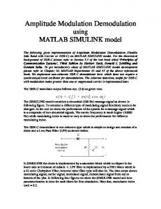
tory system (Oppenheim and Willsky 1997). Figure 1A illustrates these basic concepts from the engineering encoding perspective. Figure 1B shows the hypothesized spiking activity corresponding to neural modulation encoding (third row: PM encoding; fourth row: AM encoding) of the considered stimulus with sinusoidally modulated carrier frequency ( first row, FM) and amplitude (second row, AM). An ensemble of PM encoding neurons (third row) will produce an evoked neural PM signal similar to that shown in the middle of the bottom panel of Fig. 1A (obtained mathematically by low-pass filtering the spike train). Similarly, an ensemble of AM encoding neurons ( fourth row) will produce an evoked neural AM signal similar to that shown in the middle of the top panel of Fig. 1A. This neural modulation encoding model will be addressed in more detail in the DISCUSSION. In the Fourier domain, modulated signals have distinctive signatures, which may be easier to detect and decode than their time-domain versions. A narrowband carrier appears as a single peak in the spectrum at ƒcarrier, the carrier frequency. The modulations arising from either pure AM or pure PM appear as sideband frequency patterns in the spectrum. Specifically, the spectrum will have an upper sideband at ƒcarrier ⫹ ƒmodulation and a lower sideband at ƒcarrier ⫺ ƒmodulation (often accompanied by additional, lower-power sidebands at more distant frequencies). At least one example of modulation encoding is seen in human auditory cortex: at extremely slow frequency modulations (about 0.1 Hz), the phase of the envelope modulation frequency aSSR tracks the carrier change, i.e., a form of PM encoding (Patel and Balaban 2000, 2004). Whether other

FIG. 1. Modulation as an encoding method in engineering and proposed neural mechanisms. A: modulation signal modulates either the amplitude (AM) or the phase (PM) of the carrier signal to produce either an AM signal or a PM signal. Both signals produce a 2-sideband pattern in spectrum (right). B: possible neural modulation encoding mechanisms for AM encoding and PM encoding to simultaneously represent both stimulus carrier (1st row: changes in stimulus carrier frequency) and stimulus envelope (2nd row: changes in stimulus amplitude) dynamics. A neuron using PM encoding (3rd row) fires one spike per stimulus envelope cycle, as indicated by the dotted line, and the firing phase in each cycle depends on the instantaneous stimulus carrier frequency. A neuron using AM encoding (last row) changes firing rate according to the instantaneous stimulus carrier frequency, while keep the firing phase within each cycle fixed (aligned with the dotted line).

J Neurophysiol • VOL

96 • NOVEMBER 2006 •

www.jn.org

2714

H. LUO, Y. WANG, D. POEPPEL, AND J. Z. SIMON

methods are used—and what method is used at higher frequencies—is largely unknown. The ability of auditory cortex to track stimulus dynamics by the aSSR is limited. The aSSR to AM sounds can be recorded with MEG from humans at stimulus rates up to about 100 Hz, with a large peak around 40 Hz (Ross et al. 2000); EEG responses follow to higher rates (see, e.g., Picton et al. 2003) but responses at those higher rates are not generated by auditory cortex. The aSSR at the modulation frequency, however, is generated only by neural temporal coding, whereas many neurons use rate coding for rapidly modulated stimuli (Lu et al. 2001). Therefore it is still not fully understood how—and how fast—auditory cortex can track a stimulus, particularly for stimuli modulated in both envelope and carrier, as is typical of most ecologically relevant signals. The present study was designed to address three questions: First, how does human auditory cortex represent or corepresent simultaneous AM and FM. Second, how fast can human auditory cortex track the carrier dynamics (FM). Third, is there any coding transition as the rate of carrier dynamics increases? To address these issues, we take advantage of the high temporal resolution of MEG, which has shown to be a method with outstanding sensitivity to record from human auditory cortex.

44.1 kHz. The stimuli were sinusoidally frequency modulated tones with modulation frequencies ( ƒFM) of 0.3, 0.5, 0.8, 1.0, 1.7, 2.1, 3.0, 5.0, and 8.0 Hz and frequency deviation between 220 and 880 Hz. In addition, the entire stimulus amplitude was modulated sinusoidally at a fixed rate of 37 Hz ( ƒAM) with modulation depth of 0.8. All stimuli were 10 s in duration and shaped by rising and falling 100-ms cosine-squared ramps. Each stimulus was presented 10 times. Figure 2 shows the spectrogram (top), the spectrum (middle), and the temporal waveform (bottom) of example stimuli, confirming that the stimulus sounds contain both sinusoidally modulated temporal envelope at ƒAM (37 Hz) and sinusoidally modulated carrier frequency at ƒFM (0.8 and 2.1 Hz as examples drawn here). Because the frequency range of the carrier ranges from 220 to 880 Hz, the stimuli have the broadband spectra shown in the middle panel. To ensure that subjects attend to the long stimulus sequences, 36 distracter stimuli were created and inserted into the experiment for subjects to detect. Those distracters were the same as the normal stimuli except single short-duration FM sweeps were inserted at random time in the stimulus. Subjects were instructed to press a button when detecting the distracter stimuli. Normal stimuli (90 ⫽ 9 ⫻ 10) and distracter stimuli (36) were mixed and played in a pseudorandom order at a comfortable loudness level to subjects. Subjects performed the required task fairly well (average miss rate: about 3/36; average false alarm rate: about 1/36). The entire experiment was divided into four blocks with breaks between them. Only the data for normal stimuli were further analyzed.

METHODS

Subjects

MEG recordings

Twelve subjects (eight males) with normal hearing and no neurological disorders provided informed consent before participating in this experiment. The subjects’ mean age was 25 and all were righthanded. A digitized head shape was obtained for each subject for use in equivalent-current dipole source estimation.

Neuromagnetic signals were recorded continuously with a 157channel whole-head MEG system (5-cm baseline axial gradiometer SQUID-based sensors; KIT, Kanazawa, Japan) in a magnetically shielded room, using a sampling rate of 1,000 Hz and an on-line 100-Hz analog low-pass filter, with no high-pass filtering. Each subject’s head position was determined by five coils attached to anatomical landmarks (nasion, left and right preauricular points, two forehead points) at the beginning and the end of recording to ensure that head movement was minimal. Head shape was digitized using a three-dimensional digitizer (Polhemus).

Stimuli Nine stimuli were created, using custom-written MATLAB programs (The MathWorks, Natick, MA), with a sampling frequency of Spectrogram Frequency (Hz)

Frequency (Hz)

fFM = 0.8 Hz 1500 1000 500 0

0

2

4

6

fFM = 2.1 Hz 1500 1000 500 0

8

0

2

Time (sec)

4000

2000

2000

200

400 600 Frequency (Hz)

8

6000

4000

0

6

Time (sec)

Spectrum

6000

0

4

800

0

1000

0

200

400

600

800

1000

Frequency (Hz)

Temporal waveform

(f AM = 37 Hz)

0.4

FIG. 2. Stimulus examples. Top: spectrograms of stimuli with ƒFM equal to 0.8 and 2.1 Hz. Carrier frequency was modulated at a particular frequency (left, 0.8 Hz; right, 2.1 Hz), sinusoidally from 220 to 880 Hz. Middle: corresponding spectra of the stimulus examples in top panel (left, 0.8 Hz; right, 2.1 Hz). Note that the spectra are broadband. Bottom: temporal waveform of stimulus with ƒFM equal to 2.1 Hz. Envelope of the stimulus is modulated sinusoidally at 37 Hz. Only one segment from 0.2 to 1.4 s is shown to allow the 37-Hz AM be seen more clearly. Carrier change can also be seen here. Stimuli have both dynamic envelope (bottom) and carrier (top).

0

0. 4

0.3

0.5

0.7

0.9

1.1

1.3

Time (sec)

J Neurophysiol • VOL

96 • NOVEMBER 2006 •

www.jn.org

SIMULTANEOUS DYNAMIC ENVELOPE AND CARRIER ENCODING

Data analysis Data from 10 trials for a given condition (same ƒFM) were concatenated (total of 100 s per condition) and were discrete Fourier transformed (DFT) using 100,000 points. DFT was performed on data of all 157 MEG channels and for all nine stimulus conditions.

2715

structed to count the number of 1-kHz pure tones they heard. The M100 component is believed to originate in the superior temporal cortex on the upper bank of the superior temporal gyrus slightly posterior to Heschl’s gyrus on the planum temporale (Lutkenhoner and Steinstrater 1998). This direct comparison permits an analysis of the aSSR location without requiring MRI.

Phasor representation and channel selection

Sideband confusion matrix

For each channel, the steady-state response (aSSR) at 37 Hz ( ƒAM) is parameterized by the DFT component’s magnitude and phase at 37 Hz ( ƒAM). The result is a map of complex aSSR, i.e., a map of complex magnetic field values. An example of such a map can be seen in Fig. 3B, where the complex magnetic field at each channel is represented by a phasor, i.e., an arrow with length proportional to the complex field magnitude and with direction given by the complex field phase (Simon and Wang 2005). The 10 channels per subject with the largest magnitudes across all the channels in both hemispheres at the 37 Hz ( ƒAM) modulation frequency were regarded as channels representative of auditory cortical activity and selected for further analysis, motivated by the positive relationship between tracking performance and response strength at ƒAM found in an MEG experiment exploring representation of tone sequence in human auditory cortex (Patel and Balaban 2004).

To test for the presence of general modulation encoding, including the possibility of AM and PM encoding, we examined the spectra of the MEG responses to comodulated stimuli for a two-sideband pattern: with strong spectral peaks at ƒAM ⫾ ƒFM, a distinctive signature of modulation encoding. Target sideband frequencies were defined for different ƒFM as upper sideband ( ƒAM ⫹ ƒFM) and lower sideband ( ƒAM ⫺ ƒFM), leading to 18 (9 ⫻ 2) frequencies (upper: 37.3, 37.5, 37.8, 38, 38.7, 39.1, 40, 42, 45 Hz; lower: 36.7, 36.5, 36.2, 36, 35.3, 34.9, 34, 32, 29 Hz). The DFT amplitude and phase at every target sideband frequency were extracted for 10 channels (selected specifically per subject), for every stimulus condition, giving an 18 ⫻ 9 ⫻ 10 ⫻ 12 data set (frequency ⫻ stimulus condition ⫻ channel ⫻ subject). Confusion matrix analysis was used to assess statistical significance. In this methodology, any one particular sideband frequency is examined for all stimulus conditions (even those whose responses should not elicit the sideband). Ideally, the response to the one stimulus whose FM is at the corresponding frequency examined in the response should elicit higher magnitude at that frequency than that of all other stimuli. Then, even under noisy conditions, at a particular target sideband frequency, more channels should elicit the highest magnitude for the stimulus condition with the appropriate ƒFM than that of any other stimulus condition. For example, for the target sideband frequency of 38 Hz (37 ⫹ 1, the upper sideband for stimulus with ƒFM ⫽ 1 Hz), the stimulus with ƒFM ⫽ 1 Hz should elicit a larger number of channels with

aSSR and M100 equivalent-current dipole localization To localize the neural source of the aSSR, the complex aSSRs corresponding to ƒFM ⫽ 0.3 Hz were analyzed to determine the best (least mean square) fit for a pair of equivalent-current dipoles (Simon and Wang 2005). The resulting complex dipoles’ positions, one in each hemisphere, are the estimates of the source locations. These aSSR source locations are compared with the M100 source locations, estimated by the purely real version of the same algorithm. The M100 was measured in a pretest experiment, in which subjects were in-

A

B

x 105 8

6

4 FIG. 3. Auditory steady-state response (aSSR) at envelope modulation frequency (37 Hz). A: spectrum of the response from one representative channel of one subject. Arrow indicates the evoked aSSR at 37 Hz. B: phasor representation of aSSR at 37 Hz, clearly showing a bilateral auditory magnetoencephalography (MEG) contour map. Arrow in each channel represents the Fourier coefficient at 37 Hz. Arrow length represents the magnitude and the arrow direction represents the phase. C: grand average of dipole location for the aSSR at 37 Hz (red) and M100 (green) in axial, sagittal, and coronal views. Two dipoles are localized in similar position of superior temporal cortex.

2

0

30

34

38

Frequency (Hz)

42

C

J Neurophysiol • VOL

96 • NOVEMBER 2006 •

www.jn.org

2716

H. LUO, Y. WANG, D. POEPPEL, AND J. Z. SIMON

maximum strength at 38 Hz than that of any of the other stimuli (other ƒFM). If that is true, we claim that modulation encoding is used to corepresent the envelope and carrier dynamics characterized by ƒAM ⫽ 37 Hz and ƒFM ⫽ 1 Hz. For each target sideband frequency, the magnitudes at this frequency for all nine stimulus conditions were compared and the stimulus that elicited maximum magnitude at this sideband frequency was stored, indexed by its stimulus condition (out of nine). This calculation was performed for all target sideband frequencies (nine upper sidebands and nine lower sidebands) for all 10 of the selected channels, giving an 18 ⫻ 10 ⫻ 12 (frequency ⫻ channel ⫻ subject) analysis set. Each cell represents the index number of the stimulus condition inducing maximum response at this frequency, for each channel and each subject. Because it is possible that only one of the two sideband frequencies was detectable in the MEG signal arising from different signal-to-noise ratios, upper and lower sideband frequencies were explored separately. For each subject two separate 9 ⫻ 9 confusion matrices were constructed to represent the upper and lower sideband performance. For example, in upper sideband confusion matrix (Fig. 5A), columns represent stimuli conditions ( ƒFM of 0.3– 8 Hz) and rows represent different target upper sideband frequencies (37 ⫹ 0.3 to 37 ⫹ 8 Hz). Each element in the matrix represents the number of channels that were the largest magnitude elicited at this frequency (corresponding row) by this stimulus (corresponding column). The sum of each single row is equal to 10 (channels) and thus each row actually reflects the histogram of stimulus condition that drove the specific sideband frequency most across 10 channels. Ideally, if every sideband frequency is maximally elicited by the corresponding stimulus condition, the confusion matrix will be purely diagonal. We construct upper and lower sideband confusion matrices for each subject and also, to represent the total sideband performances, the sum of the two confusion matrices (top panels of each of the subfigures in Fig. 5 show the sum of the confusion matrix across 12 subjects). To further determine whether sidebands were significantly elicited (i.e., whether the diagonal is significantly peaked in the whole confusion matrix) and to explore differences for different stimulus conditions, the results from the diagonal axis were extracted from both the upper and the lower sideband confusion matrices for each subject. These nine-element arrays were normalized (to range from 0 to 1) and correspond to the proportion of channels that showed the correct maximum sideband for each subject (see the bottom panels of each of the subfigures in Fig. 5 for the grand averages across 12 subjects). For example, a value of 1 means that, for that target sideband frequency, the stimulus with the corresponding ƒFM elicited maximum magnitude for all channels; whereas a value of 0.2 reflects that only 20% of all the selected channels showed maximum magnitude at this target sideband frequency when the corresponding stimulus occurred. The same procedure was also applied in the total sideband confusion matrix where the data range was normalized to range from 0 to 2 so it roughly shows whether two sidebands or one sideband was elicited. A Monte Carlo simulation was used to calculate the 95% significance threshold for the proportion value for both the one-sideband confusion matrix and the total sidebands confusion matrix (dotted-starred line in the bottom panels of each of the subfigures in Figs. 5 and 6). The same confusion matrix procedure was used to investigate direct aSSR at ƒFM frequencies of 0.3– 8 Hz and is shown in Fig. 5D.

Simulations of confusion matrix performance The nine-element diagonals of the three confusion matrices in the bottom panels of Fig. 5, A–C are measures of sideband performance. They are used to determine the statistical significance of modulation encoding for different stimulus dynamics, specifically, the different FM ( ƒFM, 0.3– 8 Hz). A simulation was performed to compare the confusion matrix performance and sideband performance for pure PM encoding with the empirical results. Only the simulation of pure PM J Neurophysiol • VOL

encoding is shown, but pure AM encoding would provide similar results. Confusion matrix performance by itself cannot distinguish between the types of modulation encoding and it is only one way to check the possibility of modulation encoding. By comparing the simulation results with real MEG results, however, we are informed as to whether modulation encoding is used at all. A simulation of neural responses with pure PM encoding was created with neural carrier frequency 37 Hz ( ƒAM), neural modulation frequencies ( ƒFM) of 0.3– 8 Hz, random starting phases (␾1, ␾2), and neural modulation depth of 0.6. The simulation signals were created by adding Gaussian white noise (GWN), the level of which was adjusted to match the real neural sideband performance S PM ⫽ cos关2␲fAMt ⫹ ␾1 ⫹ 0.6 cos共2␲fFMt ⫹ ␾2兲兴 ⫹ GWN

The simulated signal results in a confusion matrix, just as for the empirical data. Block simulations represented 12 subjects, composed of the nine different ƒFM conditions, each of which was simulated 10 times (representing 10 channels). Then the confusion matrix for the higher sideband, the lower sideband, and the total sideband performance (the same frequencies as in empirical data) was calculated using the same procedures described above. These are shown in the top panels of each of the subfigures of Fig. 6. The sideband performance for each of the three confusion matrices was extracted from the diagonal of the corresponding simulated confusion matrix. These are shown in the bottom panels of each of the subfigures of Fig. 6.

Encoding-type parameter calculation Sidebands naturally occur for all types of modulation coding (including AM and PM). To help determine which modulation coding created the sidebands, an encoding-type parameter (␣, defined below, ranging between 0 and 2␲) was calculated to distinguish AM encoding from PM encoding. Both encoding mechanisms (see Fig. 1B) elicit two sidebands, but with different phase relationships across the sidebands and carrier. As will be seen below, AM encoding produces ␣ near 0 (or 2␲); PM encoding produces ␣ near ␲ (for reasonably moderate phase modulation index values). The encoding-type parameter ␣ is defined as (␪upper ⫺ ␪AM) ⫺ (␪AM ⫺ ␪lower), using, respectively, the phase at the sidebands ƒupper ⫽ ƒAM ⫹ ƒFM, ƒlower ⫽ ƒAM ⫺ ƒFM, and carrier ƒAM. The mathematical derivation follows. For neural response carrier frequency fc (identified with ƒAM), neural response modulation frequency fm (identified with ƒFM), and modulation index m, this is shown for the neural response case of AM S AM共t兲 ⫽ cos 关1 ⫹ m cos 共2␲fmt ⫹ ␾1兲兴 cos 共2␲fct ⫹ ␾2兲 ⫽ cos 共2␲fct ⫹ ␾2兲 ⫹ ⫹

m cos 关2␲共fc ⫹ fm兲t ⫹ ␾1 ⫹ ␾2兴 2

m cos 关2␲共fc ⫺ fm兲t ⫹ ␾2 ⫺ ␾1兴 2

⫽ cos 共2␲fct ⫹ ␾2兲 ⫹

m m cos 共2␲fuppert ⫹ ␪upper兲 ⫹ cos 共2␲flowert ⫹ ␪lower兲 2 2

where we have set ␪upper ⫽ ␾1 ⫹ ␾2 and ␪lower ⫽ ␾2 ⫺ ␾1. Thus ␣AM :⫽ (␾upper ⫺ ␾2) ⫺ (␾2 ⫺ ␾lower) ⫽ [(␾1 ⫹ ␾2) ⫺ ␾2] ⫺ [␾2 ⫺ (␾2 ⫺ ␾1)] ⫽ 0, which is also equivalent to ␣AM ⫽ 2␲. Correspondingly in the neural PM case S PM共t兲 ⫽ cos 关2␲fct ⫹ ␾3 ⫹ m cos 共2␲fmt ⫹ ␾4兲兴 ⫽ cos 共2␲fct ⫹ ␾3兲 cos 关m cos 共2␲fmt ⫹ ␾4兲兴 ⫺ sin 共2␲fct ⫹ ␾3兲 sin 关m cos 共2␲fmt ⫹ ␾4兲兴 ⬇ cos 共2␲fct ⫹ ␾3兲 ⫺ m sin 共2␲fct ⫹ ␾3兲 cos 共2␲fmt ⫹ ␾4兲

96 • NOVEMBER 2006 •

www.jn.org

SIMULTANEOUS DYNAMIC ENVELOPE AND CARRIER ENCODING ⬇ cos 共2␲fct ⫹ ␾3兲 ⫹ ⫹

冉

冉

冊

m ␲ cos 2␲fuppert ⫹ ␾3 ⫹ ␾4 ⫹ 2 2

冊

m ␲ cos 2␲flowert ⫹ ␾3 ⫺ ␾4 ⫹ 2 2

⬇ cos 共2␲fct ⫹ ␾3兲 ⫹

m m cos 共2␲fuppert ⫹ ␪upper兲 ⫹ cos 共2␲flowert ⫹ ␪lower兲 2 2

where we have set ␪upper ⫽ ␾3 ⫹ ␾4 ⫹ (␲/2) and ␪lower ⫽ ␾3 ⫺ ␾4 ⫹ (␲/2), giving ␣PM ⫽ (␪upper ⫺ ␾3) ⫺ (␾3 ⫺ ␪lower) ⫽ {[␾3 ⫹ ␾4 ⫹ (␲/2)] ⫺ ␾3} ⫺ {␾3 ⫺ [␾3 ⫺ ␾4 ⫹ (␲/2)]} ⫽ ␲, concluding the mathematical derivation. Experimentally, the encoding-type parameter ␣ may take either of these values or any value between, and so a distribution of measured values is expected. ␣ was calculated for all nine different ƒFM stimuli conditions, all 10 selected channels, and all 12 subjects. A histogram of ␣ distribution across channels and subjects was drawn for each ƒFM stimulus condition. It should be noted that the calculation presented for ␣PM is valid for only small modulation index m (found to be smaller than ␲/4 by Patel and Balaban 2004), but it can be shown numerically that the result is robust even for moderately large values of m (up to about 3␲).

Encoding-type parameter statistics Circular statistics were used to estimate the (circular) mean and (circular) standard error of ␣. To calculate the circular mean value ␣៮ , for each ƒFM, all the ␣ were first converted into complex vectors (ei␣) and the mean of those complex vectors was determined. The circular mean ␣៮ is the four-quadrant inverse tangent of this complex vector mean. The circular SE of ␣ (SE␣) was calculated using bootstrap (balanced, 1,000 instances) across the ␣ of all the selected channels and all 12 subjects (Efron and Tibshirani 1994; Fisher 1996).

Simulations of mixed neural PM encoding and AM encoding

2717

frequency ƒAM. Because of the limited signal-to-noise ratio in the MEG signal, other peaks (external narrowband noise) are also observable (and known not to be attributable to movement or related artifacts or to bad sensors). The relevance of using sidebands to detect neural modulation coding is that the vast majority of the noise peaks cannot interfere with the sidebands. Figure 3B shows the corresponding phasor representations for aSSR at 37 Hz for all channels (Simon and Wang 2005). There is a clear bilateral auditory cortical origin for aSSR at 37 Hz. Figure 3C shows the grand average results for both the aSSR equivalent-current dipole (red) and the M100 (green). The dipole locations of aSSR and of M100 activity were compared across all subjects, and it was found that they have displacements not significantly different from 0 (for right hemisphere: ⌬x ⫽ ⫺1.1 ⫾ 5.3 mm, ⌬y ⫽ 4.6 ⫾ 7.6 mm, ⌬z ⫽ ⫺2.4 ⫾ 5.8 mm; for left hemisphere: ⌬x ⫽ ⫺0.0 ⫾ 3.2 mm, ⌬y ⫽ 4.4 ⫾ 8.2 mm, ⌬z ⫽ ⫺4.1 ⫾ 5.4 mm). This result supports the idea that the source of aSSR is in the superior temporal cortex because the M100 component is believed to originate there (Lutkenhoner and Steinstrater 1998). This result is consistent with the aSSR localization results of Ross et al. (2000) given the resolution limitations of this data set. Auditory steady-state response at sidebands Figure 4 shows the aSSR at upper sidebands for the same channel in the same subject at different stimulus conditions. First, the aSSR at 37 Hz ( ƒAM) can be seen for all nine different stimulus conditions (black arrow); second, stimuli with specific ƒFM elicited corresponding sidebands [here, only upper sidebands are shown (gray arrows); the lower sidebands, not shown, do not necessarily follow the same pattern]. For example, for stimulus ƒFM ⫽ 0.5 Hz, the response at 37.5 Hz (⫽37 ⫹ 0.5) is elicited, and when stimulus ƒFM ⫽ 1 Hz, the

A simulation was performed to see how different neural encoding schemes using mixed AM encoding and PM encoding affect the resulting ␣ parameter distribution. The simulation results are compared with the empirical ␣ distribution data and provide suggestions for possible mechanisms for sidebands appearance in real MEG data (e.g., pure AM encoding, pure PM encoding, or mixture of AM encoding and PM encoding). Simulated pure neural AM encoding signals and PM encoding signals with carrier frequency of 37 Hz ( ƒAM) and modulation frequency of 2 Hz (one example of ƒFM) were created with random starting phase (␾i) and the simulation mixture signals were created by combining them using different weights ␶ S AM共t兲 ⫽ 关1 ⫹ 0.4 cos 共2␲fFMt ⫹ ␾1兲兴 cos 共2␲fAMt ⫹ ␾2兲 SPM共t兲 ⫽ cos 关2␲fAMt ⫹ ␾3 ⫹ cos 共2␲fFMt ⫹ ␾4兲兴 S共t兲 ⫽ ␶SAM共t兲 ⫹ 共1 ⫺ ␶兲SPM共t兲

The encoding-type parameter ␣ for this simulated signal was then calculated as above. We performed 1,000 simulations for each weight parameter ␶ that ranged from 0.1 to 0.9 in steps of 0.1 and calculated the ␣ distribution histogram for different values of ␶. RESULTS

Auditory steady-state response at fAM Figure 3A shows the discrete Fourier transform of one channel of a representative subject, including the aSSR at ƒAM (37 Hz). The spectrum shows a clear peak at 37 Hz, the AM J Neurophysiol • VOL

FIG. 4. Spectrum and aSSR at sidebands at one channel in a representative subject. Each of the 9 figures represents the spectrum for each of the 9 different ƒFM stimulus conditions. Black arrow points to the aSSR at envelope modulation frequency (37 Hz) and can be observed for all the stimulus conditions. Gray arrows indicate the aSSR at corresponding upper sideband ( ƒAM ⫹ ƒFM). For example, the stimulus with ƒFM of 0.3 Hz elicited 37.3-Hz aSSR (gray arrow). For this specific channel, all the stimulus conditions elicited corresponding upper sidebands except the stimulus with ƒFM of 5 Hz (gray arrow). (Subject R0458).

96 • NOVEMBER 2006 •

www.jn.org

2718

H. LUO, Y. WANG, D. POEPPEL, AND J. Z. SIMON

response at 38 Hz (⫽37 ⫹ 1) is elicited. For this one channel, the upper sideband for ƒFM of 5 Hz is not visible. Note that narrowband noise coexists with the sidebands we want to detect. Sideband performance Figure 5 shows the sum of confusion matrices across all subjects. We can see that for both upper and lower sideband confusion matrices (Fig. 5, A and B), most rows peak on the diagonal, reflecting that the stimulus did strongly elicit responses at the upper and lower sideband frequencies. Figure 5C is the sum of upper and lower confusion matrices across all

subjects and also clearly shows the peaks along the diagonal. The curve below each confusion matrix is the corresponding diagonal value vector and the starred line is the 95% threshold. The total sideband performance (Fig. 5C) is well above the threshold for all the stimuli we tested here. There is some difference between upper and lower sideband performances (Fig. 5, A and B). Specifically, the poor performance in the upper sideband for the two lowest values of ƒFM is artifactual, arising from the strong narrowband system noise at the corresponding upper sideband frequencies (37.3 and 37.5 Hz), but present for almost all channels and all subjects. The narrowband noise at those two frequencies can be seen for all nine conditions in Fig. 4 and clearly masks any elicited sidebands at those frequencies.

FIG. 5. Empirical confusion matrix performance across 12 subjects. A: upper sideband confusion matrix. B: lower sideband confusion matrix. C: total sideband confusion matrix. D: ƒFM confusion matrix. In the confusion matrix, each box represents the number of channels that elicited maximum magnitude at a particular sideband frequency (vertical axis) by a given stimulus condition (horizontal axis), for all stimulus conditions. Each row actually represents the histogram of best-driving stimulus for this specific sideband, and the sum of one row is equal to 120 (10 total channels ⫻ 12 subjects). If a particular sideband is significantly elicited by its corresponding stimulus, in one row (for one sideband frequency), the response on the diagonal will dominate the row. Peaked diagonal for all 4 confusion matrices can be seen here. Plot underlying each confusion matrix is the diagonal value plot normalized by channel number and subject number for the corresponding confusion matrix. For Fig. 4, A, B, and D, the intensity reflects the response frequency’s performance; because only one response frequency is tabulated, the range is from 0 (no aSSR at this frequency elicited at all) to 1 (aSSR elicited for all 10 channels and all 12 subjects). For C, because upper and lower sideband performances are summed, the range intensity is from 0 to 2 (2 sideband frequencies elicited for all 10 channels and all 12 subjects). Generally, the diagonal values are above the threshold line, showing significant aSSR at these frequencies (sideband frequencies or ƒFM frequencies).

J Neurophysiol • VOL

96 • NOVEMBER 2006 •

www.jn.org

SIMULTANEOUS DYNAMIC ENVELOPE AND CARRIER ENCODING

Simulation of confusion matrix and sideband performance The simulation results (Fig. 6, A–C) can be compared with the experimental results (Fig. 5, A–C), to demonstrate to what extent that modulation encoding is be used. As can be seen in Figs. 5A and 6A, the upper sideband performance of real MEG data matches well with the simulation (except for ƒFM of 0.3 and 0.5 Hz, which was discussed above, can arise as an artifact as a result of the narrowband noise at 37.3 and 37.5 Hz). The empirical lower sideband performance matches well with the simulated lower sideband performance (Figs. 5B and 6B) for ƒFM ⬍ 5 Hz. Considering upper and lower sideband performances together, as reflected in empirical total sideband per-

2719

formance (Figs. 5C and 6C), we can confirm that modulation encoding is used for the entire ƒFM range tested here (0.3– 8 Hz). The deteriorated performance for lower sideband performance for ƒFM ⬎ 5 Hz may have arisen from some kind of encoding transition, but because the performance for the upper sideband is still above threshold during that range (Fig. 5A), this demonstrates that some form of modulation encoding is present (even if not pure PM or pure AM encoding). Auditory steady-state response at fFM The significance of the responses at the ƒFM (i.e., not at the corresponding sidebands of ƒAM) was explored using the same

FIG. 6. Simulated confusion matrix and sideband performance for a response using pure PM encoding with added Gaussian noise, assuming the same noise level and modulation index across all 9 conditions. Noise level is adjusted to match the empirical results. Sideband performance was extracted from the corresponding simulated confusion matrices and is shown below each confusion matrix. Dotted-starred line is the 95% threshold from a Monte Carlo simulation. A: top sideband confusion matrix. B: lower sideband confusion matrix. C: total sideband confusion matrix. Approximate match between empirical data (Fig. 5, A–C) and simulated data (A–C) reflects modulation encoding.

J Neurophysiol • VOL

96 • NOVEMBER 2006 •

www.jn.org

2720

H. LUO, Y. WANG, D. POEPPEL, AND J. Z. SIMON

confusion matrix procedure. Figure 5D shows the confusion matrix for the actual ƒFM frequencies (not sidebands elicited around ƒAM). and we can see that most of the stimuli, especially the stimuli with higher ƒFM (⬎0.5 Hz) showed aSSR at the corresponding ƒFM frequency. Encoding-type parameter ␣ Figure 7A shows the ␣ histograms for different ƒFM. For lower ƒFM (⬍5 Hz), the ␣ distribution is peaked and centered near or at ␲ (the PM encoding region), except at 0.3 Hz. For the highest ƒFM (5 and 8 Hz), ␣ shows a more uniform-like distribution between 0 and 2␲. In addition,

using circular statistics, the mean and SE of the encodingtype parameter ␣ are shown in Fig. 7B for different ƒFM. The gray bars define the PM encoding region, ␲ ⫹ (␲/4), and AM encoding region, within ␲/4 of 0 or 2␲ (the range is arbitrary and for illustrative purposes only). For the lower ƒFM range ( ƒFM ⬍ 5 Hz, except at 0.3 Hz), the encodingtype parameter ␣ is near ␲ and within the PM encoding region. As ƒFM increases, ␣ begins to leave the PM encoding region, but at the same time becomes more uniformly distributed and the bootstrap derived circular error of the mean becomes larger. The uniform-like distribution for ƒFM of 0.3 Hz is also explained by the narrowband noise at the upper sideband frequency (37.3 Hz), which in turn leads to a noisier encoding parameter distribution.

FIG. 7. Encoding-type parameter ␣ performance. A: ␣ histogram across the 10 selected channels and all 12 subjects for different stimulus conditions. Dotted line indicates the circular mean of ␣. Both figures show that for stimulus with lower ƒFM (⬍5 Hz), ␣ is centered around ␲ and thus in the PM encoding region. When ƒFM becomes faster, ␣ becomes more uniformly distributed and also leaves the PM encoding region. B: ␣ plot for different stimulus condition. Mean of ␣ is calculated using circular statistics. SE is calculated using bootstrap across all channels and subjects. Gray bar represents the PM encoding region (the middle gray bar, around ␲) and the AM encoding region (the top and bottom gray bars, around 0 or 2␲).

J Neurophysiol • VOL

96 • NOVEMBER 2006 •

www.jn.org

SIMULTANEOUS DYNAMIC ENVELOPE AND CARRIER ENCODING

Simulation of ␣ dependency on neural AM and PM encoding mixtures As stated in the INTRODUCTION, the spectral sideband can arise from a variety of modulation encodings, including AM encoding: the amplitude of aSSR at ƒAM (37 Hz) tracking the carrier frequency change. A simulation demonstrates whether additional involvement of AM encoding can account for the observed ␣ distribution for higher ƒFM (⬎5 Hz). Figure 8 shows the ␣ distribution for different mixtures. As can be seen, when the AM encoding contribution is very small (e.g., ␶ ⫽ 0.1), so that the coding is dominated by PM encoding, ␣ is narrowly distributed around ␲. When the AM encoding contribution ␣ is increased and thus the signal is a more balanced mixture of AM encoding and PM encoding, ␣ approaches a more uniform distribution (␶ ⫽ 0.5, 0.6). When the AM encoding contribution ␶ is large (e.g., ␶ ⫽ 0.9), the signal is dominated by AM encoding and ␣ peaks around 0 (or 2␲). Comparing the simulation results with our experimental results, we see that the ␣ distribution for lower ƒFM (⬍5 Hz) is similar to the simulation results with small AM encoding weight ␶ (0.1– 0.3), although the simulation has a narrower distribution. This supports a model of PM encoding dominance at lower ƒFM rates. Interestingly, in our results for higher ƒFM (5 and 8 Hz), the ␣ distribution is more uniform, which looks like the simulations with AM encoding and PM encoding mixed in similar proportions. This suggests that the experimental results for higher ƒFM may be attributable to involvement of additional AM encoding. DISCUSSION

2721

fixed envelope dynamics ( ƒAM ⫽ 37 Hz), and varied the carrier dynamics. We explored the possibility that auditory cortex corepresents the envelope and carrier dynamics simultaneously using modulation encoding by determining whether a spectral sideband pattern is elicited. In addition, by changing the carrier dynamics from slow to fast (0.3– 8 Hz), we investigated the possibility of a coding transition (PM encoding vs. AM encoding). Relationship to previous aSSR findings Consistent with previous research (Ross et al. 2000), we find a robust aSSR at ƒAM (37 Hz here), which means auditory cortex demodulates the incoming sound and extracts the envelope. The aSSR at ƒFM is consistent with EEG studies using pure frequency-modulated stimuli (Picton et al. 1987), which is one way auditory cortex represents pure carrier dynamics, although they tested much higher modulation frequencies (⬎80 Hz) than those used here. Dimitrijevic et al. (2001) used independent amplitude and FM (IAFM) stimuli with also higher-modulation frequencies and found separate AM and FM aSSR responses that are relatively independent of each other, suggesting separate and independent encoding of envelope and carrier. We also found the aSSR at ƒFM, but because our AM frequency was fixed, we cannot estimate whether the aSSR at ƒAM and ƒFM were independent of each other. When the source of the aSSR was localized using equivalent-current dipoles, no significant difference was found between the location of these dipoles and those of the (well-studied) M100. Sidebands and modulation encoding

Human auditory cortex encodes a sound’s envelope dynamics (AM), as well as its carrier frequency dynamics (FM). To investigate the way auditory cortex represents different carrier dynamics, we used a specifically designed acoustic stimulus, a sinusoidally comodulated stimulus with

FIG. 8. Simulation of ␣ distributions using different proportions of neural AM and PM encoding. Neural AM and PM signals were created using same modulation (2 Hz) and carrier frequency (37 Hz). Neural signals were simulated as the sum of AM encoding (weight ␶) and PM encoding (weight 1 ⫺ ␶). ␣ was calculated for each of the 1,000 simulation trials and their distributions are shown for different ␶ (0.1 to 0.9 in step of 0.1). Small ␶ corresponds to dominant PM encoding and large ␶ corresponds to dominant AM encoding, when ␶␣ has a quasi-uniform distribution.

J Neurophysiol • VOL

Spectral sideband patterns were found throughout our results, either in the upper sideband or lower sideband confusion matrix, indicating that auditory cortex does use modulation encoding to simultaneously corepresent envelope and carrier dynamics. The detection of the spectral sideband pattern alone, however, does not determine the particular type of modulation encoding (e.g., PM vs. AM). Note that the stimuli used here to probe the cortical response differ only in FM rates, from slow to moderately fast, sharing all other properties: common spectral widths, envelope dynamics (37 Hz), and temporal structure (simultaneous AM and FM), as shown in Fig. 2. Therefore the response transition found in this study reflects a cortical transformation and cortical encoding scheme change, as a function of only FM dynamics. The weak sideband performance in the upper sideband confusion matrix (Fig. 5A) for ƒFM of 0.3 and 0.5 Hz is probably a result of the narrowband noise at these two sideband frequencies (37.3 and 37.5 Hz), which in turn gives lower signal-to-noise ratios at these points. Figure 4 shows the spectrum for one channel under all nine stimulus conditions, and the narrowband noise at 37.3 and 37.5 Hz can be clearly seen for all the stimulus conditions. The same reason accounts for the noisy distribution of encoding-type parameter ␣ for ƒFM of 0.3 Hz because the phase calculated at this frequency point is also affected by noise. For stimuli with faster-changing carriers ( ƒFM ⱕ 8 Hz), the upper sideband is consistently significant, which supports the use of modulation encoding by human auditory cortex to simultaneously represent the envelope and carrier dynamics.

96 • NOVEMBER 2006 •

www.jn.org

2722

H. LUO, Y. WANG, D. POEPPEL, AND J. Z. SIMON

To distinguish between types of modulation encoding used (e.g., AM encoding vs. PM encoding), we analyzed the distribution of the encoding-type parameter ␣, which is approximately ␲ for pure PM encoding and approximately 0 or 2␲ for pure AM encoding (Fig. 8). We found that for slower ƒFM stimuli (⬍5 Hz, excluding the 0.3 and 0.5 Hz upper sidebands), the encoding-type parameter ␣ is approximately ␲ (Fig. 7), indicating that those sidebands are attributed to the phase modulation of ƒAM by ƒFM. In other words, the phase of the aSSR at ƒAM tracked the stimulus carrier frequency change and, because the carrier frequencies changed at certain frequencies ( ƒFM), the phase of ƒAM also changed at the corresponding ƒFM frequencies. These results for slower ƒFM were consistent with Patel and Balaban (2000) where the phase of the aSSR reliably tracked the carrier frequency contour of the tone sequences. There the carrier was a long, periodic series of concatenated tone segments ( ƒFM ⬵ 0.1 Hz), rather than the sinusoidally modulated carrier in our experiment. These results suggest that for stimuli with slow carrier dynamics ( ƒFM ⬍ 5 Hz), auditory cortex tracks the carrier dynamics, i.e., the stimulus carrier frequency change, by modulating the phase of the aSSR at ƒAM accordingly. As ƒFM increases, ␣ begins to deviate from ␲ (Fig. 7), indicating that encoding by phase tracking alone begins to deteriorate. Because upper sidebands are still present for those higher ƒFM stimuli (Fig. 5A), modulation encoding (PM or AM or, e.g., both PM and AM) is still used. One possibility is that another class of neurons have been recruited that use the amplitude, rather than the phase, of the aSSR at ƒAM to track the carrier dynamics. This kind of mechanism of AM encoding also elicits two sidebands around ƒAM, but producing an encoding-type parameter ␣ of nearly 0 (or 2␲), as shown in our simulation (Fig. 8). We will explain this possibility in detail. Possible modulation coding schemes Patel and Balaban (2004) proposed a model to explain their phase tracking results. They suggest that there are two groups of neurons, both of which fire in a phase-locked fashion to the envelope of the stimulus. One group of neurons tracks the carrier change by varying the firing phase within each ƒAM cycle, whereas the other group of neurons has only uniform random phase variation, although they still fire phase locked to the ƒAM envelope. Using this model, the observed phasetracking results can be explained by reasonable neuronal mechanisms, specifically, the first group of neurons. This leads directly to responses dominated by PM encoding. We propose another possible neural response type: the AM encoding neuron. These neurons also fire in a phase-locked fashion to the envelope of the stimulus ( ƒAM), but they change the firing rate rather than the firing phase within each cycle of ƒAM to track the carrier frequency change. Such kind of neuron group can elicit two sidebands around ƒAM with encoding-type parameter ␣ around 0 (or 2␲). The two proposed neuronal types are depicted in Fig. 1B. In this illustrated example, the PM encoding neuron (third row) fires earlier for higher stimulus carrier frequency ( first row) and fires later for lower stimulus carrier frequency (shown by the distance between the spike and the dotted line). In contrast, the AM encoding neuron ( fourth row) in this example fires at J Neurophysiol • VOL

a higher rate for higher stimulus carrier frequency and at a lower rate for lower stimulus carrier frequency. Lu et al. (2001) found two largely distinct populations of neurons in auditory cortex of awake marmosets: one with stimulus-synchronized discharge (temporal code) coding for slow sound patterns and the other using a rate code for rapidly repeating events. They suggest that the combination of temporal and rate codes provides a possible neural basis for wide range of temporal information representation in auditory cortex. Consistent with their suggestions, it is also possible that two groups of neurons, the PM encoding-type and the AM encoding-type neurons, are simultaneously involved in encoding envelope and carrier dynamics, and that the proportions depend on the stimulus dynamics. Single-population models using both PM and AM are also possible and not ruled out by these results. For stimuli with low ƒFM, more PM encodingtype neurons are involved (temporal coding) and, as ƒFM increases, more AM encoding-type neurons begin to join, tracking carrier dynamics by AM (rate) coding. MEG signals reflect combinations of responses from (potentially) many different neuronal classes. Therefore when AM encoding neurons become involved in encoding stimulus dynamics, the observed MEG signals will be the sum of responses from both PM encoding-type and AM encoding-type neuronal responses. This affects the encoding-type parameter ␣ distribution, as shown in the simulation results (Fig. 8): the mixture of encoding populations causes the distribution to become more uniformly (broadly) distributed, rather than narrowly centered at ␲ (for pure PM encoding). Saberi and Hafter (1995) proposed an FM-to-AM transduction hypothesis whereby a change in frequency is transmitted as a change in amplitude and suggested a common neural code (temporal code) for AM and FM sounds. In contrast, Moore and Sek (1996) suggested a two-stage FM sound-detection mechanism: the FM detection at low rate mainly depends on temporal information (phase locking to the carrier), whereas FM detection at higher rates (⬎10 Hz) depends mainly on changes in the excitation pattern (a “place” mechanism). Although both refer to pure FM detection, the ideas apply straightforwardly to our suggested interpretations. In general, our results provide support for simultaneous encoding of envelope and carrier dynamics by modulation encoding in human auditory cortex. For stimuli with slow carrier dynamics (⬍5 Hz), pure PM encoding is used. For stimuli with faster carrier dynamics (here ⱕ8 Hz), modulation encoding is still present but probably not pure PM encoding. We propose the hypothesis that another group of neurons using AM encoding will be involved and continue to represent the stimulus dynamics. Importantly, our results provide natural hypotheses and predictions that can be tested in further neurophysiological studies. ACKNOWLEDGMENTS

We are grateful to J. Walker for excellent technical assistance and to three reviewers for thoughtful and detailed comments. GRANTS

H. Luo, Y. Wang, and D. Poeppel were supported by National Institute on Deafness and Other Communication Disorders Grant R01 DC-05660 to D. Poeppel.

96 • NOVEMBER 2006 •

www.jn.org

SIMULTANEOUS DYNAMIC ENVELOPE AND CARRIER ENCODING REFERENCES

Ahissar E, Nagarajan S, Ahissar M, Protopapas A, Mahncke H, and Merzenich MM. Speech comprehension is correlated with temporal response patterns recorded from auditory cortex. Proc Natl Acad Sci USA 98: 13367–13372, 2001. Boemio A, Fromm S, Braun A, and Poeppel D. Hierarchical and asymmetric temporal sensitivity in human auditory cortices. Nat Neurosci 8: 389 –395, 2005. Dimitrijevic A, John MS, van Roon P, and Picton TW. Human auditory steady-state responses to tones independently modulated in both frequency and amplitude. Ear Hear 22: 100 –111, 2001. Doupe AJ and Kuhl PK. Birdsong and human speech: common themes and mechanisms. Annu Rev Neurosci 22: 567– 631, 1999. Drullman R, Festen JM, and Plomp R. Effect of temporal envelope smearing on speech reception. J Acoust Soc Am 95: 1053–1064, 1994. Efron B and Tibshirani RJ. An Introduction to the Bootstrap. London: Chapman & Hall/CRC, 1994. Eggermont JJ. Temporal modulation transfer functions for AM and FM stimuli in cat auditory cortex. Effects of carrier type, modulating waveform and intensity. Hear Res 74: 51– 66, 1994. Elhilali M, Fritz JB, Klein DJ, Simon JZ, and Shamma SA. Dynamics of precise spike timing in primary auditory cortex. J Neurosci 24: 1159 –1172, 2004. Fisher NI. Statistical Analysis of Circular Data. Cambridge, UK: Cambridge Univ. Press, 1996. Gaese BH and Ostwald J. Temporal coding of amplitude and frequency modulation in the rat auditory cortex. Eur J Neurosci 7: 438 – 450, 1995. Giraud AL, Lorenzi C, Ashburner J, Wable J, Johnsrude I, Frackowiak R, and Kleinschmidt A. Representation of the temporal envelope of sounds in the human brain. J Neurophysiol 84: 1588 –1598, 2000. Heil P and Irvine DR. Functional specialization in auditory cortex: responses to frequency-modulated stimuli in the cat’s posterior auditory field. J Neurophysiol 79: 3041–3059, 1998. John MS and Picton TW. Human auditory steady-state responses to amplitude-modulated tones: phase and latency measurements. Hear Res 141: 57–79, 2000. Liang L, Lu T, and Wang X. Neural representations of sinusoidal amplitude and frequency modulations in the primary auditory cortex of awake primates. J Neurophysiol 87: 2237–2261, 2002. Liegeois-Chauvel C, Lorenzi C, Trebuchon A, Regis J, and Chauvel P. Temporal envelope processing in the human left and right auditory cortices. Cereb Cortex 14: 731–740, 2004. Lu T, Liang L, and Wang X. Temporal and rate representations of timevarying signals in the auditory cortex of awake primates. Nat Neurosci 4: 1131–1138, 2001. Lutkenhoner B and Steinstrater O. High-precision neuromagnetic study of the functional organization of the human auditory cortex. Audiol Neurootol 3: 191–213, 1998.

J Neurophysiol • VOL

2723

Moore BC and Sek A. Detection of frequency modulation at low modulation rates: evidence for a mechanism based on phase locking. J Acoust Soc Am 100: 2320 –2331, 1996. Oppenheim AV and Willsky AS. Signals and Systems. Englewood Cliffs, NJ: Prentice-Hall, 1997. Patel AD and Balaban E. Temporal patterns of human cortical activity reflect tone sequence structure. Nature 404: 80 – 84, 2000. Patel AD and Balaban E. Human auditory cortical dynamics during perception of long acoustic sequences: phase tracking of carrier frequency by the auditory steady-state response. Cereb Cortex 14: 35– 46, 2004. Picton TW, John MS, Dimitrijevic A, and Purcell D. Human auditory steady-state responses. Int J Audiol 42: 177–219, 2003. Picton TW, Skinner CR, Champagne SC, Kellett AJ, and Maiste AC. Potentials evoked by the sinusoidal modulation of the amplitude or frequency of a tone. J Acoust Soc Am 82: 165–178, 1987. Rees A, Green GG, and Kay RH. Steady-state evoked responses to sinusoidally amplitude-modulated sounds recorded in man. Hear Res 23: 123–133, 1986. Ross B, Borgmann C, Draganova R, Roberts LE, and Pantev C. A high-precision magnetoencephalographic study of human auditory steadystate responses to amplitude-modulated tones. J Acoust Soc Am 108: 679 – 691, 2000. Saberi K and Hafter ER. A common neural code for frequency- and amplitude-modulated sounds. Nature 374: 537–539, 1995. Schreiner CE and Urbas JV. Representation of amplitude modulation in the auditory cortex of the cat. I. The anterior auditory field (AAF). Hear Res 21: 227–241, 1986. Schreiner CE and Urbas JV. Representation of amplitude modulation in the auditory cortex of the cat. II. Comparison between cortical fields. Hear Res 32: 49 – 63, 1988. Shannon RV, Zeng FG, Kamath V, Wygonski J, and Ekelid M. Speech recognition with primarily temporal cues. Science 270: 303–304, 1995. Simon JZ and Wang Y. Fully complex magnetoencephalography. J Neurosci Methods 149: 64 –73, 2005. Smith ZM, Delgutte B, and Oxenham AJ. Chimaeric sounds reveal dichotomies in auditory perception. Nature 416: 87–90, 2002. Viemeister NF. Temporal modulation transfer functions based upon modulation thresholds. J Acoust Soc Am 66: 1364 –1380, 1979. Wang XQ, Lu T, and Liang L. Cortical processing of temporal modulations. Speech Commun 41: 107–121, 2003. Zatorre RJ, Belin P, and Penhune VB. Structure and function of auditory cortex: music and speech. Trends Cogn Sci 6: 37– 46, 2002. Zeng FG, Nie K, Stickney GS, Kong YY, Vongphoe M, Bhargave A, Wei C, and Cao K. Speech recognition with amplitude and frequency modulations. Proc Natl Acad Sci USA 102: 2293–2298, 2005. Zwicker E. Die Grenzen der Horbarkeit der Amplitudenmodulation und der Frequenzmodulation eines Tones. Acustica 2: 125–133, 1952.

96 • NOVEMBER 2006 •

www.jn.org