Conditional Expectations and Renormalization

arXiv:math-ph/0204038v1 17 Apr 2002

Conditional Expectations and Renormalization Alexandre J. Chorin Department of Mathematics University of California Berkeley, CA 94720 Abstract In optimal prediction methods one estimates the future behavior of underresolved systems by solving reduced systems of equations for expectations conditioned by partial data; renormalization group methods reduce the number of variables in complex systems through integration of unwanted scales. We establish the relation between these methods for systems in thermal equilibrium, and use this relation to find renormalization parameter flows and the coefficients in reduced systems by expanding conditional expectations in series and evaluating the coefficients by Monte-Carlo. We illustrate the construction by finding parameter flows for simple spin systems and then using the renormalized (=reduced) systems to calculate the critical temperature and the magnetization.

Key words: Conditional expectations, optimal prediction, renormalization, parameter flow, critical exponents, spins, averaging.

1

1

Introduction

In the optimal prediction (OP) methods presented in earlier work by the author and others [7],[5],[8],[4], an estimate of the future solution of an underresolved problem, or of a problem where the initial data are only partially known, was obtained by solving a reduced system of equations for the conditional expectation of the solution given the partial data. This system, closely related to a generalized Langevin equation of the Mori-Zwanzig type [9],[15], is derived in detail in [6]. Short-time estimates can be obtained by keeping only the first term on the right hand side of this system, obtaining a relation between the rate of change of a reduced set of variables and conditional expectations of the full rate of change; a simplified derivation of this relation is given below. Hald’s theorem [5] asserts that if one starts with a Hamiltonian system, then the reduced system obtained in this way is also Hamiltonian, with a Hamiltonian equal to a conditional free energy of the original Hamiltonian system. Renormalization group (RNG) transformations [3],[12],[13] reduce the dimensionality of a system of equations by integrating out unwanted scales. That there is a qualitative resemblance between OP and RNG methods is quite clear, and has been pointed out in particular in the related work of Goldenfeld et al. [10],[11]. In the present paper we focus on the special case of Hamiltonian systems in thermal equilibrium, and show that in this case the RNG transformations of the Hamiltonian can be obtained by integrating conditional expectations of the derivatives of the Hamiltonian; loosely speaking, RNG transformations are integrals of OP reductions. This remark, based on Hald’s theorem, makes possible the efficient evaluation of the coefficients of the new Hamiltonians in RNG transformations (the “RNG parameter flow”) by simple Monte-Carlo methods, for example by Swendsen’s small-cell Monte-Carlo RNG [3],[14]. The coefficients in the new Hamiltonian define the reduced system of equations used to estimate the future in OP. To illustrate the construction, we apply it to spin systems and obtain explicitly the parameter flows in addition to critical points, critical exponents, and order parameters. We exhibit in detail a particular implementation that is a little awkward if viewed as an instance of a RNG but is particularly convenient for OP. A little thought shows that what is offered in the present paper is a numerical short-cut. Suppose x = (x1 , x2 , . . .) is a set of n random variables (n may be infinite), and let m < n; partition x so that x = (ˆ x, x ˜), x ˆ = (x1 , x2 , . . . , xm ), x ˜= (xm+1 , xm+2 , . . .). Let p = p(x) be the joint probability density of all the ˆ = H(ˆ ˆ x) such that variables, and consider the problem of finding a function H Z ˆ x)) = p(x)d˜ exp(−H(ˆ x, (1) 2

ˆ is well defined but the where d˜ x = dxm+1 dxm+2 · · ·. There is no question that H obvious ways of finding it can be costly. We are offering effective ways to do so. There are other situations where one wants to integrate out unwanted variables inside nonlinear functions, and our short-cut may serve there as well; in subsequent papers we shall apply it to problems in irreversible statistical mechanics and, equivalently, to problems involving the full long-time OP equations.

2

Conditional expectations and optimal prediction

Consider a set x of random variables (x1 , x2 , . . . , xn ) with a joint probability R density of the form Z −1 e−H(x) , Z = e−H(x) dx, dx = dx1 dx2 . . . dxn . Consider the space L2 of function u(x), v(x), . . ., with the inner product hu, vi = E[uv] = R u(x)v(x)Z −1 exp(−H)dx, where E[·] denotes an expected value. Partition the variables into two groups as above, x = (ˆ x, x ˜), xˆ = (x1 , . . . , xm ), m < n. Given a function f (x), its conditional expectation given x ˆ is Z f (x)e−H(x) d˜ x E[f (x)|ˆ x] = Z ; (2) e−H(x) d˜ x it is the average of f keeping x ˆ fixed. The conditional expectation is a function of x ˆ only, and it is the best approximation of f in the mean square sense by a function of xˆ: i i h h 2 2 (3) x)) E (f (x) − E[f (x)|ˆ x]) ≤ E (f (x) − h(ˆ

for any function h = h(ˆ x). E[f |ˆ x] is the orthogonal projection of f onto the ˆ 2 of L that contains functions of x subspace L ˆ only. E[f (x)|ˆ x] can be approxiˆ mated by expansion in a basis of L2 ; keeping only a suitable finite number ℓ of basis functions ϕ1 (ˆ x), ϕ2 (ˆ x), . . . , ϕℓ (ˆ x), and minimizing the distance between f and the span of the ϕi (ˆ x), one finds E[f |ˆ x] =

ℓ X

ci ϕi (ˆ x),

i=1

where the ci satisfy the equation Φc = r,

3

(4)

where Φ is the matrix with elements Φij = hϕi , ϕj i, c = (c1 , . . . , cℓ ), and r = (hf, ϕ1 i, hf, ϕ2 i . . . , hf, ϕℓ i). Usually the inner products can be calculated by Metropolis sampling. ˆ = H(ˆ ˆ x) such that Suppose you want to find a function H Z ˆ e−H(ˆx) = e−H(ˆx,˜x) d˜ x, (5) i.e., write the marginal probability density of the variables x ˆ in exponential form. Suppose one can write H(x) =

ℓ X

αi ϕi (x),

i=1

and and let i ≤ m, where m is the number of components of the vector x ˆ = Then Z ∂ H(x)e−H(x) d˜ x h i ∂x ∂ i Z E H(x)|ˆ x = ∂xi (6) e−H(x) d˜ x
∂ − log R e−H(x) d˜ x . = ∂x i An analogous relation between the derivative of a logarithm of a partially integrated density and a conditional expectation arises also in the context of expectation-maximization is statistics [1]. ˆ 2 consisting of functions of the form ∂ ϕj (ˆ If one can find a basis for L x), ∂x1 j = 1, . . . , and provided the set of variables so that for all h is homogenous i P ℓ ∂ H|ˆ ∂ ϕ (ˆ i ≤ m the coefficients cj in the expansions ∂x x = j=1 cj ∂x j x) are i i independent of i, then the expansion X ˆ x) = H(ˆ cj ϕj (ˆ x). (7) follows immediately. This is our key observation. This construction is just Hald’s theorem for OP [5]: Suppose one has a system of differential equations (written as ordinary differential equations for simplicity) of the form d ϕ(t) = R (ϕ(t)) , ϕ(0) = x dt

(8)

where ϕ, R and x are n-vectors with components ϕi , Ri , xi , i = 1, . . . , n and t ˆ R), ˜ where ϕˆ is the time. Suppose we partition as above ϕ = (ϕ, ˆ ϕ), ˜ R = (R, contains the first m components of ϕ, etc. Suppose the system (8) is Hamiltonian, i.e., m, n are even, Ri = ∂ H for i even, Ri = − ∂ H for i odd; ∂xi−1 ∂xi+1 4

H = H(x) is the Hamiltonian and Z −1 e−H is then an invariant probability density for the system. Suppose we can afford to solve only m < n of the equations in (8) or have only m data components x ˆ. We want to solve equations for ϕ: ˆ dϕˆ ˆ = R(ϕ), ϕ(0) ˆ =x ˆ, dt ˆ is the whole vector ϕ. It is natural to where i ≤ m, but the argument of R ˆ approximate Ri (ϕ) by the closest function of ϕˆ for each i ≤ m, i.e., solve dϕˆ ˆ = E[R(ϕ) | ϕ]. ˆ dt

(9)

The approximation (9) is valid only for a short time, as one can see from the dϕˆ in [5],[6], see also below. Hald’s theorem dt ˆ = H(ˆ ˆ x) = asserts that the system (9) is Hamiltonian, with Hamiltonian H R −H(x) ˆ − log e d˜ x, a relation identical to equation (6). The existence of H shows that the approximation (9) cannot be valid for long times: the predictive power of partial initial data decays at t → ∞ for a nonlinear system, and the best estimate of ϕ(t) ˆ should decay to unconditional mean of ϕ (which is usually zero). The existence of a reduced Hamiltonian shows that this decay can happen only to a limited extent and thus the approximation can in general be valid only for short times. Equations (9) constitute the short time, or “first-order”, OP approximation. Suppose however that instead of picking specific values for the initial data x ˆ ˆ one samples them from the invariant density Z −1 e−H(ˆx) . The distribution of the x ˆ’s is then invariant, and equal to their marginal distribution in the full system (8) when the data are sampled from the invariant distribution Z −1 e−H(x) , as R
R ˆ = exp log e−H d˜ one can also see from the identities exp(−H) x = e−H d˜ x. The system (9) then generates the marginal probability density of part of the variables of a system at equilibrium. Thus OP at equilibrium is a way of reducing the number of variables without affecting the statistics of the variables that remain. One can make short-time predictions about the future from the reduced system with coefficients computed at equilibrium because it is self-consistent to assume for short times that unresolved degrees of freedom are in thermal equilibrium, as is explained in the OP papers cited above. full equation for the evolution of

3

Renormalization

For simplicity, we work here with real-space renormalization applied to variables associated with specific sites in a plane, x(1) = (xI1 , xI2 , . . .), where Ik = (ik , jk ), 5

ik , jk are integers, all the Ik are inside a square D of side N with N large, and the variables are listed in some convenient order. The Hamiltonian H = H (1) is a function of x(1) , H (1) = H (1) (x(1) ). The need for the superscript (1) will R (1) (1) appear shortly. We assume that the partition function Z = e−H (x ) dx(1) (1) (1) is well defined, where dx(1) = dxI1 dxI2 . . .. Suppose we group the variables xI1 , xI2 , . . . into groups of ℓ variables (for example, we could divide D into squares each containing 4 variables). The variables can be referred to as “spins”in conformity with common usage in (2) (2) physics. Associate with each group a new variable xJ1 , xJ2 , . . . , where J1 , J2 , . . . (2)

is some ordering of the new variables and xJk is a function (not necessar(2)

(2) ily invertible) of the xI in (1) (1) (1) g(xIm+1 , xIm+2 , . . . , xIm+ℓ ) for (2) (2) (xJ1 , xJ2 . . .). We can write

Z

= = (2)

R

R

e−H

(2)

dx

(2)

(1)

the group labeled by Jk , for example xJk = the appropriate m. The vector x(2) is x(2) =

(x(1) )

R

dx(1) (2)

δ x

(1)

− g(x


−H (1) (x(1) ) (1) . ) e dx

where dx(2) = dxJ1 dxJ2 · · · , and the δ function is a product of delta functions, one per group. If one defines H (2) (x(2) ) by the equation Z   (1) −H (2) (x(2) ) e = δ x(2) − g(x(1) ) e−H(x ) dx(1) , (10) R (2) (2) then Z = e−H (x ) dx(2) . The mapping x(1) → x(2) , followed by a change of numbering of the remaining variables so that J1 , J2 . . . (the indices of the new variables x(2) ) enumerate the new variables by going through all integer pairs in a reduced domain of side √ N/ ℓ, is a real-space renormalization group transformation; it produces a new set of variables which has less spatial detail than the previous set and such that √ distances between the remaining spins have been scaled down by ℓ. If the calculation is set up so that the mapping x(1) → x(2) , H (1) → H (2) can be repeated, for example, if the range of the variables x(1) is invariant and the Hamiltonians H (1) , H (2) can be represented in the same finite-dimensional basis, then one can produce in this way a sequence of Hamiltonians H (1) , H (2) , H (3) , . . .; the fixed points of the transformation H (n) → H (n+1) for a spin system of infinite spatial extent include the critical points of the system, see any discussion of the RNG, for example [12],[13]. (1) (2) Consider the special case where xJ is one of the xI in its group–i.e., replace a block of spins by one of the spins in the block. More general and widely used assignments of block variables will not be needed in the present paper and will 6

be discussed elsewhere. We can identify the spins that remain with x ˆ of the preceding section and the spins that disappear with x ˜. Equation (10) becomes a special case of equation (5), and can be solved for H (2) by taking conditional expectations of the derivatives of H (1) . Note that the usual RNG representation of a renormalized Hamiltonian by means of additional couplings [12] is interpreted here as an expansion of a conditional expectation in a convergent series. The new interpretation may be useful both in understanding what is happening on the computer and in deriving error estimates. The relation between the RNG and conditional expectations shows that the latter can be calculated recursively, as we show in the example below. We have written the RNG transformation above in notation suitable for spins with a continuous range. The case of discrete (e.g., Ising) spins is automatically included, even though it may seem odd to differentiate functions with a discrete domain and range. Indeed, add to the Hamiltonian H a term of the form   1 X Y ψ(xi − x0j ) ε i j

where ε is small, the sum is over all spins, the product is over a finite number of values x0j , and ψ ≥ 0 has a minimum at 0 and is positive elsewhere. For small ε such a term will constrain the xi to take on the values x0j , but since at the origin the derivative of ψ is zero the calculation of the conditional expectations is unaffected by this term and the limit ε → 0 can be taken without actually doing anything on the computer. All one has to do is make sure that in the MonteCarlo sampling only the values x0j are sampled. Indeed, results below will be given for Ising spins which take on the values +1 and −1, with a “bare” (unP renormalized) Hamiltonian H (1) = β xI xJ , with summation over locations I, J that are neighbors on the lattice; β = 1/T , where T is the temperature.

4

A decimation RNG/OP scheme for a spin system

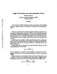
We consider in detail a RNG/recursive OP scheme where the number of variables is halved at each step. The spins are located on a square lattice with nodes Ik = (ik , jk ), ik , jk integers, and at each step of the recursion those for which ik + jk is odd are eliminated while those for which ik + jk is even are kept. The spins with ik + jk even constitute x ˆ and the others x ˜; the choice of which are even and which are odd is a matter of convention only (see Figure 1). The variables are labeled by Ik : xI1 , xI2 , . . .. 7

Figure 1: The decimation pattern Given a location I = (i, j), we group the other variables according to their distance from I: group 1 contains only xI , the variable at I. Group 2 (relative to I) contains those variables whose distance from I is 1, group 3 contains those √ variables whose distance to I is 2, etc. We form the “collective” variables 1 X Xk,I = xJ nk group k

where nk is the number of variables in the group (1 for group 1, 4 for group 2, etc.). From these variables one can form a variety of translation-invariant polyP P P nomials in x of various degrees: I xI Xk,I = I X1,I Xk,I , I (Xk,I )2 (Xk+1,I )2 , P 4 I (Xk,I ) , . . .. In practice the domain over which one sums must be finite, and it is natural to impose periodic boundary conditions at its edges to preserve the translation invariance. We wrote out explicitly only polynomials of even degrees because the Hamiltonians we consider are invariant under the transformation x → −x. The translation-invariant polynomials built up from the Xk,I can be labeled ϕ1 (x), ϕ2 (x), . . . in some order. Expand the n-th renormalized Hamiltonian in a series and keep the first ℓ terms: ℓ X (n) H (n) = αk ϕk (x). (11) k=1

The derivative of this series at the spin xI is ℓ

X (n) ∂ H (n) = αk ϕ′k (x), ∂xI 1

ϕ′k =

The functions ϕ′k are easily evaluated, for example: !′ X xJ Xk,J = 2Xk,I J

8

∂ ϕk . ∂xI

(12)

X

(Xk,J )4

J

!′



X

= 4

group k



x3J  /n2k ,

etc., where “group k” refers to distances from I, the variable with respect to which we are differentiating (see Figure 2). Pick a variable xI in xˆ (i.e., I = (i, j), i + j even in our conventions). Some of the functions ϕ′k in (12) will be functions of xˆ only and some will be functions of both x ˆ and x ˜ or of x ˜ only. The task at hand is to project the latter on the former and then rearrange the series so as to shrink the scale of the physical domain. To explain the construction we consider a very special case. Suppose one can write (n)

(n)

(n)

H (n) (x) = α2 ϕ2 + α3 ϕ3 + α4 ϕ4 ,

(13)

where ϕk (x) = xI Xk,I for k = 2, 3, 4, . . .. Note that ϕ′k = ∂x∂ I ϕk is a function only of xˆ when k = 3, 4 (and when k = 6, as we shall need to know shortly) but not when k = 2 or 5 (see Figures 1, 2). We now calculate the conditional expectations of the derivatives of H (n) given xˆ by projecting them on the space of functions of xˆ. First we project ϕ′2 on the span of ϕ′3 , ϕ′4 , ϕ′6 (note that ϕ′6 is not in the original expansion (13)). Form the matrix Φ with rows hϕ′k , ϕ′3 i, hϕ′k , ϕ′4 i, hϕ′k , ϕ′6 i for k = 3, 4, 6, the primes once again denoting differentiation with respect to xI . Form the vector r with component (hϕ′2 , ϕ′3 i, hϕ′2 , ϕ′4 i, hϕ′2 , ϕ′6 i). Let c = (c1 , c2 , c3 ) be the solution of Φc = r (see equation (4)). The coefficients c are the coefficients of the orthogonal projection ˆ 2 . After projection, the of ϕ′2 onto the span of ϕ′3 , ϕ′4 , ϕ′6 which is contained in L coefficients of ϕ3 , ϕ4 in (13) become P

(n)

(n)

(n)

(n)

= α3 + α2 c1 , αnew 3 αnew = α4 + α2 c2 , 4 (n)

and ϕ6 acquires the coefficient α2 c3 . If one relabels the remaining spins so that they occupy the lattice previously occupied by all the spins, group 3 becomes group 2, group 4 becomes group 3, and group 6 becomes group 4 (see Figure 2). The new Hamiltonian H (n+1) now has the representation (n+1)

H (n+1) = α2 with

(n+1)

ϕ2 + α3

(n+1)

ϕ3 + α4

(n)

(n)

(n)

(n)

(n+1)

= α3 + α2 c1 ,

(n+1)

= α4 + α2 c2 ,

(n+1)

=

α2 α3 α4

(n)

α2 c3 . 9

ϕ4 ,

7

7

6

5

4

5

6

5

3

2

3

5

4

2

I

2

4

5

3

2

3

5

6

5

4

5

6

7

7

Figure 2: The collective variables More generally, if H (n) is expressed as a truncated series, partition the terms in ∂ the series for ∂x H (n) into functions of x ˆ and functions of both x ˆ and x ˜. Add I to the terms which are functions of x ˆ additional terms which are functions of x ˆ and are chosen so that after relabelling they acquire the form of terms already in the series (just as above, terms that depend on X3,J , for example, become terms that depend on X2,J after relabelling). Project the functions of x on the span of the expanded set of functions of x ˆ, collect terms and relabel. This is a renormalization step, and it can be repeated. Note that it if one wants to reduce the number of variables by a given factor, one can in principle use an analogous RNG/conditional expectation construction and get there in one iteration; the recursive construction is easier to do and the intermediate Hamiltonians, whose coefficients constitute the parameter flow in the renormalization, contain useful information. The discussion so far may suggest that one sample the Hamiltonians recursively, i.e., start with H (1) , find H (2) , use Monte-Carlo to sample the density (2) Z −1 e−H and find H (3) etc. The disadvantages of this approach are: (i) The (n) sampling of the densities Z −1 e−H can be much more expensive for n > 1 than for n = 1 because each proposed Monte-Carlo move may require that ∂ the full series for ∂x H (n) be summed twice; and (ii) each evaluation of a new I Hamiltonian is only approximate because the series are truncated, and, more important, the Monte-Carlo evaluation of the coefficients may have limited accuracy. These errors accumulate from step to step and may produce false fixed points and other artifacts. The remedy lies in Swendsen’s observation [3],[14] that the successive Hamiltonians can be sampled without being known explicitly. Sample the original Hamiltonian, remove the unwanted spins and relabel the remaining spins so as to cover the original lattice, as in the relabelling step in the renormalization; 10

(2)

the probability density of the remaining spins is Z −1 e−H ; repeating n times (n+1) yields samples of Z −1 e−H . The price one pays is that to get an m by m (n) sample of Z −1 e−H one has to start by sampling a 2q m by 2q m array of nonrenormalized spins, where q is either (n + 1)/2 or n/2 depending on the parity of n and on programming choices; the trade-off is in general very worthwhile. What has been added to Swendsen’s calculation is an effective evaluation of the coefficients of the expansion of H (n) from the samples. The programming here requires some care. With the decimation scheme as in Figure 1, after one removes the unwanted spins in x(n) the remaining spins, √ the variables x(n+1) , live on a lattice with a mesh size 2 larger than before; after relabelling they find themselves on a lattice with the same mesh size as before but arranged at a π/4 angle with respect to the previous lattice. To extract a square array from at this set of spins one has to make the size of the box that includes all the spins half the size of the previous box. At the next renormalization one obtains x(n+2) which can be extracted from x(n) by taking one spin in four and the resulting box size is the same as the size of the box that contains x(n+1) . One may worry a little about boundary conditions for x(n+1) : the periodicity of x(n) is not the same as the periodicity one has to assume for x(n+1) because of the rotation; the resulting error is too small to be detected in our calculations.

5

Some numerical results

We now present some numerical results obtained with the RNG/conditional expectation scheme. The problem we apply the construction to is Ising spins; more interesting applications will be presented elsewhere. The point being made is that the construction can be effectively implemented. The results are presented for Ising spins. (n) In table I we list the coefficients αk in the expansion of H (n) for n = 1, . . . 7 and T = 2.27. The functions ϕk are as follows: X ϕk = xJ Xk,J for k = 1, 2, 3, 4, 5, 6 ϕ6+k =

X

(Xk+1,J )4 , for k = 1, 2, 3 X 2 2 ϕ10 = X2,J X3,J .

Note that as a result of the numbering of the ϕ’s the last coefficient is not necessarily the smallest coefficient. This table represents the parameter flow and if the functions ϕk are written in terms of the variables xJ the table defines the new system of equations for the reduced set of variables. Remember that 11

ˆ 2 additional functions are used so that after relabelling in the projection on L the series has the same terms , but maybe with different coefficients, as before the renormalization. In H (1) , α2 is the sole non-zero coefficient, and its value is determined by T and the definition of X2,J , in particular the presence of the coefficient n2 (see above). It is instructive to use the parameter flow to identify the critical temperature Tc . For T < Tc the renormalization couples ever more distant spins while for T > Tc the spins become increasingly decoupled. One can measure the increasing or decreasing coupling by considering the quadratic terms in the P Hamiltonian (the terms of the form xJ Xk,J ) and calculating the “second (n) moments” M2 of their coefficients αk : (n)

M2

=

ℓ X

(n)

d2k αk

k=2

where dk is the distance from J of the spins in the group k (see the definition of P (n) Xk,J ), αk is the coefficient of xJ Xk,J in the expansion of H (n) , and ℓ is the number of quadratic terms in this expansion. In Figure 3 we show the evolution (n) of M2 with n for various values of T (with ℓ = 5 and 7 functions over-all in the expansion, including non-quadratic functions). 5

T=1.8 T=2.0 T=2.15 T=2.20 T=2.30 T=2.50

4.5

4

3.5

3

2.5

2

1.5

1

0.5

0

0

1

2

3

4

5

Figure 3: Second moments of the coefficients of the renormalized Hamiltonian for various values of T for successive iterations (n)

In Figure 4 we show the evolution of M2 near Tc = 2.269 . . . with ℓ = 6 and 10 terms in the expansion. The non-uniform behavior of M2 is not a surprise (it 12

is related to the non-uniform convergence of critical exponents already observed by Swendsen). Each step in the renormalization used 105 Monte-Carlo steps per spin. From these graphs one would conclude that Tc ∼ 2.26, an error of .5%. The accuracy depends on the number of terms in the expansion and on the choice of terms; with only 6 terms (4 quadratic and 2 quartic), the error in the location of Tc increases to about 3%. The point is not that this is a good way to find Tc but that it is a check on the accuracy of the parameter flow. From the Table one can see that the system first approaches the neighborhood of a fixed point and then diverges from it, as one should expect in a discrete sequence of transformations. 2.6

2.4

2.2

2

1.8

1.6

1.4

T=2.24 T=2.25 T=2.26 T=2.27 T=2.28 T=2.29

1.2

1

0.8

0

1

2

3

4

5

Figure 4: Second moments of the coefficients of the renormalized Hamiltonian near Tc

13

Parameter iteration α1 α2 α3 α4 α5 α6 α7 α8 α9 α10

Table 1 flow for the Ising model T = 2.26, 10 basis functions 1 2 3 4 5 6 7 0 .26 .35 .44 .48 .52 .54 .893 .47 .47 .35 .30 .25 .21 0 .32 .20 .23 .21 .20 .18 0 .04 .08 .11 .12 .13 .13 0 .07 .11 .13 .13 .12 .12 0 −.01 .01 .01 .02 .03 .02 0 −.08 −.07 −.10 −.09 −.09 −.08 0 .04 .02 .02 .01 .00 −.10 0 −.00 −.01 −.00 −.00 .00 .00 0 −.12 −.17 −.18 −.18 −.17 −.16

0.9

0.8

0.7

0.6

0.5

0.4

0.3

0.2

0.1

0 2.1

20 x 20 40 x 40 60 x 60 20 x 20, renormalized Onsager 2.15

2.2

2.25

2.3

2.35

2.4

2.45

Figure 5: Bare and renormalized magnetization near Tc We now use the renormalized system to calculate the magnetization m = P E[ xI /n2 ]. To get the correct non-zero m for T < Tc on a small lattice the symmetry must be broken, and we do this by imposing on all the arrays the boundary condition xboundary = 1 rather than the periodic boundary conditions used elsewhere in this paper. In Figure 5 we display m computer with the bare (unrenormalized) Hamiltonian H (1) on 3 lattices: 20 by 20, 40 by 40, 60 by 60, as well as the results obtained on a 20 by 20 lattice by sampling the density defined by the renormalized Hamiltonian H (5) which corresponds in principle to an 80 by 80 bare calculation. We also display the exact Onsager values of m. 14

The calculations focus on values of T in the neighborhood of Tc where the size of the lattice matters; one cannot expect the results to agree perfectly with the Onsager results on a finite lattice with periodic boundary conditions for any n; all one can expect is to have the values of the small renormalized calculation be consistent with results of a larger bare calculation. We observe that they do, up to the shift in Tc already pointed out and due to the choice of basis functions. The determination of the critical exponents for a spin model is independent of the determination of the coefficients in the expansion of H (n) , and is mentioned here only because it does provide a sanity check on the constructions, in particular on the adequacy of the basis functions. For comparable earlier calculations, see in particular Swendsen’s chapter in [3]. As is well known, if A (n) (n+1) /∂αj at T = Tc , those of its eigenvalues is the matrix of derivatives ∂αi that are larger than 1 are the critical exponents of the spin system [12]. The matrix A can be found from the chain rule [2],[3] i X ∂α(n+1) ∂E[ϕ (x(n+1) )] h  k (n+1) i = x E ϕ k (n) (n) (n+1) ∂αj ∂αj ∂αi i ∂

and the sum is over all the coefficients that enter the expansion. The derivatives of the expectations are given by correlations as follows: ∂E[ϕk (x(n+1) )] (n)

∂αj

∂E[ϕk (x(n+1) )] (n+1)

∂αi

h i = E ϕk (x(n+1) )ϕj (x(n) ) − E[ϕk (x(n+1) )]E[ϕj (x(n) )],

h i = E ϕk (x(n+1) )ϕi (x(n+1) ) − E[ϕk (x(n+1) )]E[ϕi (x(n+1) )],

see [3]. In most of the literature on real-space renormalization for Ising spins the variables x(n+1) are obtained from x(n) by “majority rule”, i.e., by assigning to the group that defines x(n+1) the value +1 if most of the members of the group are +1, the value −1 if most of the members of the group are −1, with ties resolved at random. For the decimation scheme described above our “pick one” rule (x(n+1) is one of the members of the group) is identical to the majority rule. There is an apparent difficulty in the decimation because at each recursion the number of terms in the summation that defines the basis functions is reduced by half while the square root of an integer is not in general an integer, so that one has to perform Swendsen sampling on rectangles so designed that the ratio of the areas of two successive rectangles is 1/2. This has not turned out to be harmful, and the value of ν, the correlation exponent, was found to be 1 (the exact value) ±.01 with 106 Monte-Carlo moves per spin, the error depending mainly on the number of Monte-Carlo moves which has to be very large, in line 15

with previous experience [14]. We also checked that in a renormalization scheme where a 2 × 2 block of spins is replaced at each iteration by a single spin, the “majority rule” and our “pick one” rule for x(n+1) yield similar results. One needs fewer terms in the expansion of the Hamiltonian to get accurate values of the exponents than to get an accurate parameter flow, but a larger number of Monte-Carlo moves.

6

Conclusions

We have presented a simple relation between conditional expectations for systems at equilibrium on one hand and the RNG on the other, which makes it possible to find efficiently the coefficients in a reduced systems of equations for a subset of variables whose distribution as given by reduced system equals their marginal distribution in the original system. The numerical results above emphasized the neighborhood of the critical point in the simple example because this is where the variables are strongly coupled without separation of scales and a reduction in system size requires non-trivial tools. The next steps will be the application of these ideas to time-dependent problems and to finite-difference approximations of underresolved partial differential equations, along the lines suggested in [10]; this work will be presented elsewhere. Acknowledgments. I would like to thank Prof. G.I. Barenblatt, Prof. N. Goldenfeld, Prof. O. Hald, Prof. R. Kupferman, Mr. K. Lin, and Mr. P. Stinis for very helpful discussions and comments. This work was supported in part by the Office of Science, Office of Advanced Scientific Computing Research, Mathematical, Information, and Computational Sciences Division, Applied Mathematical Sciences Subprogram, of the U.S. Department of Energy under Contract No. DE-AC03-76SF00098 and in part by the National Science Foundation under grant number DMS89-19074.

16

References [1] P. Bickel and K. Doksum, Mathematical Statistics: Basic Ideas and Selected Topics, Prentice-Hall, New York, 2000, p. 133 and ff. [2] J. Binney, N. Dowrick, A. Fisher, and M. Newman, The Theory of Critical Phenomena, The Clarendon Press, Oxford, 1992. [3] T. Burkhardt and J. van Leeuwen, Real-Space Renormalization, Springer, Berlin, 1982. [4] A. Chorin, Stochastic Methods in Applied Mathematics and Physics, Lecture notes, UC Berkeley Math. Dept., 2002. [5] A. Chorin, O. Hald and R. Kupferman, Optimal prediction and the MoriZwanzig representation of irreversible processes. Proc. Nat. Acad. Sc. USA, 97, (2000), pp. 2968–2973. [6] A. Chorin, O. Hald and R. Kupferman, Optimal prediction with memory, Physica D, 2002. [7] A. Chorin, A. Kast and R. Kupferman, Optimal prediction of underresolved dynamics, Proc. Nat. Acad. Sc. USA, 95 (1998), pp. 4094–4098. [8] A. Chorin, R. Kupferman and D. Levy, Optimal prediction for Hamiltonian partial differential equations, J. Comput. Phys., 162, (2000), pp. 267–297. [9] D. Evans and G. Morriss, Statistical Mechanics of Nonequilibrium Liquids, Academic, London, 1990. [10] N. Goldenfeld, A. McKane and Q. Hou, Block spins for partial differential equations, J. Stat. Phys., 93, (1998), pp. 699–714. [11] Q. Hou, N. Goldenfeld and A. McKane, Renormalization group and perfect operators for stochastic differential equations, Phys. Rev. E, 63 (2001), pp. 036125:1–22. [12] L. Kadanoff, Statistical Physics: Statics, Dynamics, and Renormalization, World Scientific, Singapore, 2000. [13] S.S. Ma, Modern Theory of Critical Phenomena, Benjamin, Reading, Mass, 1976. [14] R. Swendsen, Monte-Carlo renormalization group, Phys. Rev. Lett. 42 (1979), pp. 859–861.

17

[15] R. Zwanzig, Nonlinear generalized Langevin equations, J. Stat. Phys., 9, (1973), pp. 215–220.

18