The resulting ODT evolution of ξg and Ys was used to assess ... In turbulent fires, knowledge of the joint soot-temperature pdf is not readily obtained. One class ...
Center for Turbulence Research Proceedings of the Summer Program 2006
311
Conditional-moment closure with differential diffusion for soot evolution in fire By J. C. Hewson†, A. J. Ricks‡, S. R. Tieszen†, A. R. Kerstein¶ A N D R. O. Foxk The conditional-moment closure (CMC) equation for the evolution of a large Lewis number scalar, soot, is derived starting from the joint probability density function (pdf) equation for the gas-phase mixture fraction, ξg , and the soot mass fraction, Ys . Unlike previous approaches starting with the joint pdf, the residual terms that result from the typical closure models were retained. A new formulation of the one-dimensional turbulence (ODT) model suitable for spatially evolving flows with buoyant acceleration and radiative transport in participating media was employed to carry out simulations of a prototypical ethene fire. The resulting ODT evolution of ξg and Ys was used to assess the significance of various terms in the CMC equation including the residual correlations. The terms involving differential diffusion are found to be important along with the soot source terms and the large-scale evolution of both ξg and Ys . Of particular importance in the regions in mixture-fraction space around the soot production and consumption is a residual term, not previously identified, related to the correlation between the differential diffusion and Ys . This term results in a diffusion-like behavior of Ys in the mixture fraction coordinate that has an apparent Lewis number near unity. In scenarios where the large Lewis number component is a non-negligible component of the mixture fraction (i.e., large soot loading), it is found easier to employ a mixture fraction neglecting this component. Such a mixture-fraction variable has a chemical source term, but this appears easier to model than the differential diffusion and dissipation terms that result when the large Lewis number component is retained in the mixture-fraction definition.
1. Introduction Soot plays a significant role in the hazard posed by hydrocarbon fires. In fires, heat transfer by radiation is the dominant means by which fires spread and cause damage. The primary source of radiant heat flux is thermal emissions from soot. Furthermore, the primary in-fire sink for radiant flux is also soot. All soot is capable of emitting and absorbing radiative flux, and the relative degree to which any soot does emit or absorb is a function of the soot-temperature distribution. Therefore, the net radiative flux in fires depends on the quantity of soot present and its joint probability density function (pdf) with temperature. In turbulent fires, knowledge of the joint soot-temperature pdf is not readily obtained. One class of approaches that can be used to approximate this quantity is the conservedscalar modeling approach. This approach is based on the idea that the thermochemical state can be referenced to a reduced set of variables for which the pdf is easier to predict. † ‡ ¶ k
Fire Science and Technology, Sandia National Laboratories, Albuquerque, NM School of Mechanical Engineering, Purdue University, West Lafayette, IN Reacting Flow Research, Sandia National Laboratories, Livermore, CA Department of Chemical and Biological Engineering, Iowa State University, Ames, IA
312
J. C. Hewson et al.
In non-premixed combustion, this reduced variable is the mixture fraction, the fraction of the local mixture that originated from the fuel source. If the pdf of the mixture fraction can be obtained and if the temperature and soot can be obtained as a function of the mixture fraction, then the joint soot-temperature pdf is obtained. There are two general frameworks for deriving conserved-scalar modeling approaches: conditional moment closure (CMC) (Klimenko & Bilger 1999) and unsteady-laminar flamelet models (ULFM) (Pitsch et al. 1998)). In the limit in which all of the transport coefficients are equal, both approaches are relatively straightforward and have been employed successfully in many studies. When species diffusivities differ, additional complications arise in the formulation. A model for flamelets with full differential diffusion has been derived by Pitsch and Peters (1998), but in the application to jet flames the best agreement with scalar fields was obtained by switching from full differential diffusion to unity Lewis numbers at the end of the jet potential core (Pitsch et al. 1998). For CMC, Kronenburg and Bilger (1997) developed a model to account for the effects of differential diffusion based on the analysis of direct numerical simulations. This model retains the different diffusivities of the species, but provides a restorative term that tends to move species profiles closer to that which would be obtained with equal diffusivities; evaluation of this term requires the solution of additional transport equations for each differentiallydiffusing scalar. For flames with soot in which differential diffusion is important, results have been reported by both Pitsch et al. (2000) and Kronenburg and Bilger (2000). Here, we reexamine the modeling of differential diffusion and identify an alternate model for addressing the effects of differential diffusion. This model does not require the solution of an additional transport equation and further explains the transition to unity Lewis numbers observed by Pitsch et al. (1998). To evaluate conserved-scalar modeling approaches and to develop new closure models, we employ a new spatially-evolving formulation of the one-dimensional turbulence (ODT) model. Within the ODT model the reaction and diffusion processes relevant to the mixture fraction, enthalpy and soot evolution are fully resolved, while the non-linear turbulent advection is modeled as a stochastic process as described by Kerstein (1999). The ODT model provides a data set for a priori evaluation of the terms in the CMC equations as it is derived here. Unique to ODT is the ability to span the range of length scales (sub-millimeter to meters) and the range of time scales (sub-millisecond to seconds) relevant to fire problems. This large range of scales arises because of the need to resolve the flame-scale chemical source terms for soot while simultaneously allowing the buoyant acceleration to drive the mixing process to fully turbulent flow and capturing the observed large-scale evolution of soot and enthalpy in fires.
2. Theory In this section the basic conservation equations for the soot evolution and the mixturefraction evolution are provided in the form in which they are used in the ODT simulations. Based on these equations, CMC equations are then derived. 2.1. Soot and mixture fraction evolution Soot evolution is modeled using a simplified two-equation treatment that retains sufficient physics for the present purposes. Equations for the soot mass fraction, Ys , ∂ρYs + ∇ · (ρ~v Ys ) − ∇ · (ρDs ∇Ys ) − ∇ · (ρDT Ys ∇ ln T ) = ρws ∂t
(2.1)
CMC with differential diffusion for soot
313
and the soot number density, which evolves similarly, are evolved. Here, ρ is the density, ~v is the velocity vector, Ds is the soot diffusivity, T is the temperature, DT = 0.75µ/[ρ(1 + παT /8)] is the thermophoretic diffusion coefficient, µ is the dynamic viscosity, αT is the thermal accommodation coefficient, and ws is the source term for soot mass fraction taken from the empirical model of Fairweather et al. (1992). The source terms are evaluated using a steady-flamelet approximation based on the mixture fraction and enthalpy. The mixture fraction can be expressed in terms of the element mass fractions that originated in the fuel stream. The element mass fraction is expressed in terms of the Pn species mass fractions, Yi , as βk = i=1 ψi,k Yi , where k is an element and ψi,k is the mass fraction of element k in species i. For the present purposes we employ elemental carbon and hydrogen to define the mixture fraction so that the mixture fraction is defined as ξ = (βC + βH )/βf where the normalization by the fuel-stream values of βC + βH is denoted βf . A common diffusion coefficient, Dξ , is selected for the mixture fraction, but not all of the species share this diffusion coefficient. Accounting for the differing diffusivities of the various species leads to a source term in the mixture-fraction conservation equation. Generally, the differential-diffusion source term on the right-hand side is negligible in hydrocarbon combustion. However, in fires and other scenarios the mass fraction associated with the particle phase is a substantial fraction of the mixture fraction, so it is necessary to include this term. For the special case where ξ = ξg + Ys /βf and where ξg is the mixture fraction contribution from the gaseous species that are all assumed to have diffusion coefficients Dξ , the conservation equation for ξ is ∂ρξ + ∇ · (ρ~v ξ) − ∇ · (ρDξ ∇ξ) = ∇ · [ρ(Ds − Dξ )∇Ys + ρDT Ys ∇ ln T ] /βf . (2.2) ∂t It turns out that the CMC equations derived using this mixture-fraction conservation equation are more challenging to model because of the differential-diffusion terms on the right-hand side. The reason for these difficulties will be discussed in Section 4. Because of these difficulties, an alternative formulation based only on the gas-phase mixture fraction is considered. The evolution equation for ξg is ∂ρξg + ∇ · (ρ~v ξg ) − ∇ · (ρDξ ∇ξg ) = −ρws . (2.3) ∂t The soot source term appears in this equation, but it is found here that the modeling of this term is more straightforward and accurate than the modeling of the differential diffusion terms. 2.2. Conditional-moment closure equations for soot There are two approaches to deriving the CMC equations. The method proposed originally by Bilger (1993), decomposing the variables into conditional means and fluctuations, was employed by Kronenburg and Bilger (1997) to analyze differential diffusion and then to study soot evolution in jet flames (Kronenburg et al. 2000). In the present work, we derive the CMC equation following the alternate method of Klimenko (1990) that is based on the joint-pdf evolution equation. The derivation from the joint-pdf equation yields the unclosed terms in different forms that provide additional insight into the issues that arise in differential diffusion. The joint-pdf equation is obtained in a standard manner using the conservation equations for the soot and the mixture fraction; Klimenko and Bilger (1999) provide an exposition for the equal-diffusivity, variable-density and inhomogeneous-flow case from
314
J. C. Hewson et al.
which the mechanistic details can be obtained. The CMC equation for Ys is obtained from the joint pdf by multiplying by Ys and integrating across all variables of the joint pdf except for the mixture fraction to obtain an equation for the marginal pdf of just the mixture fraction, fξg , and the conditional soot mass fraction � ∂ hρYs |ηi fξg + ∇ · hρ~v Ys |ηi fξg = h ρws | ηi fξg (2.4) ∂t � � ∂ 2 �
− 2 ρDs (∇ξg )2 Ys η fξg ∂η � ∂ � + h 2ρDs (∇Ys ∇ξg )| ηi fξg ∂η � ∂ h ∇ · [ρ(Dξ − Ds )∇ξg ] Ys | ηi fξg − ∂η � ∂ hρws Ys |ηi fξg /βf + ∂η + h ∇ · (ρDT Ys ∇ ln T )| ηi fξg � � +∇2 h ρDs Ys | ηi fξg − ∇ · h ∇(ρDs Ys )| ηi fξg ,
where the notation < ·|η > indicates conditional averaging with the sample-space variable η (i.e., fξg (η)). The terms on the right-hand side (r.h.s.) represent the conditional averages of contributions from the soot source term, the product of the dissipation and Ys , the ξg -Ys cross dissipation, the differential diffusion, the source of ξg from Eq. (2.2), thermophoresis and the diffusion of the pdf (two terms). Up to this point, Eq. (2.4) is an exact equation. Since the majority of the terms involve unknown correlations between various variables, a useful form of the equation requires some modeling assumptions. The conditional averages of density, Ys , the scalar dissipation rate and the diffusion velocity are defined for convenience
� ρη = hρ|ηi Qs = hYs |ηi χη = 2Dξ (∇ξg )2 |η Mη = h∇ · (Dξ ∇ξg )|ηi . (2.5)
For the second and third terms on the r.h.s., Klimenko and Bilger (1999) suggest the closures � ρ η χη Q s
ρη χη ∂Qs h 2ρDs (∇Ys ∇ξg )| ηi ≈ . (2.6) ρDs (∇ξg )2 Ys η ≈ 2Les Les ∂η
The first of these is exact if there is no correlation between the dissipation and the scalar while the second is exact if the scalar gradient is perfectly correlated with the mixturefraction gradient by ∇ξg = ∇Ys ∂Qs /∂η. The analogous approximations for the fourth and fifth terms are � � Dξ − D s ρ η M η Q s h∇ · [ρ(Dξ − Ds )∇ξg ]Ys |ηi ≈ (2.7) Dξ 2 hρws Ys |ηi ≈ hρws |ηi Qs (2.8) It is also common to separate the mean and fluctuating components of the scalar flux � � � ∇ · hρ~v Ys |ηi fξg = ∇ · hρ~v |ηi Qs fξg + ∇ · hρ~v ys0 |ηi fξg (2.9)
The terms on the last two lines of Eq. (2.4) are found to be small at reasonably large Reynolds numbers and are not discussed further. While the approximations in Eqs. (2.6) and (2.7) are suitable for many cases, we in-
CMC with differential diffusion for soot
315
vestigate here the degree to which relaxing these assumptions will lead to improved predictions in the present case where the scalar evolution is strongly affected by differential diffusion. In doing so we introduce three residual correlation terms: � � � ∂2
ρ η χη Q s 2 RDS = ρDs (∇ξg ) Ys η fξg − f ξg (2.10) ∂η 2 2Les � � ∂ ρη χη ∂Qs fξ RCD = (2.11) h 2ρDs (∇Ys ∇ξg )| ηi fξg − ∂η Les ∂η g � � � � ∂ Dξ − D s ρ η M η Q s fξg . (2.12) RDD = h∇ · [ρ(Dξ − Ds )∇ξg ]Ys |ηi fξg − ∂η Dξ 2 Using Eqs. (2.5)–(2.12) in Eq. (2.4) along with the mathematical identity � �
� � � ∂ ∂ 2 ρ η χ η f ξg − ∇ · ρDξ ∇fξg η , ρ η M η f ξg = 2 ∂η ∂η 2
(2.13)
the CMC equation for soot mass fraction is
� ∂ hρYs |ηi fξg + ∇ · hρ~v |ηi Qs fξg = h ρws | ηi fξg (2.14) ∂t 2 ρ η χ η f ξg ∂ Q s + 2Les ∂η 2 � � ∂ 2 ρ η χ η f ξg − 2 Qs ∂η 2 � � � � Dξ − Ds ∂ ρη χη fξg ∂Qs − Dξ ∂η 2 ∂η � ∂ + hρws |ηi Qs fξg /βf ∂η −RDS + RCD − RDD � −∇ · hρ~v ys0 |ηi fξg + h ∇ · (ρDT Ys ∇ ln T )| ηi fξg � � +∇2 h ρDξ Ys | ηi fξg − ∇ · h ∇(ρDξ Ys )| ηi fξg .
3. The one-dimensional turbulence model The ODT model of Kerstein (1999) is employed to evolve the mixture fraction (Eq. (2.3)), enthalpy, soot mass fraction (Eq. (2.1)) and number density conservation equations over larger length and time scales than accessible with direct numerical simulations while simultaneously resolving the reaction and diffusion processes. This is done to create a flowfield relevant to buoyant fires as a means of estimating the relative contributions of the terms in Eq. (2.14) in fire environments. Within ODT a reaction-diffusion equation is solved along a one-dimensional computational domain that may be thought of as a material line through a flowfield. The reduction of the computational domain to a single spatial dimension enables the resolution (along that domain) of the full range of length scales from the largest scales of the fire to the Kolmogorov and Corrsin scales. A model is employed to mimic the nonlinear effects of three-dimensional turbulent mixing. Despite of the reduction to 1-D of the computational
316
J. C. Hewson et al.
2
2 y (m)
3
y (m)
3
1
0 −1
1
0 x (m)
1
0 −1
0 x (m)
1
Figure 1. The evolution of the horizontal ODT domain in the vertical direction results in the depicted soot volume fraction (left) and temperature (right) fields for a single typical realization.
domain, ODT has been shown to reproduce many characteristics of three-dimensional turbulence (Kerstein 1999). Turbulent mixing is mimicked in ODT by stochastic stirring events called triplet maps, first introduced in the Linear Eddy Model of turbulent mixing, on a 1-D domain (Kerstein 1991). A triplet map increases gradients and transfers fluctuations to higher wave numbers without changing the integral fluxes of conserved scalars or introducing discontinuities in the solution. Triplet maps are the ODT analog of eddies in a turbulent flowfield. To reproduce turbulent scalings in ODT, map occurrences are based on an eddy-rate model. Eddy rates are calculated based on the energy available in the evolved velocity and density fields (Kerstein 1999). ODT has been applied to reacting-flow problems by Echekki et al. (2001) and Hewson and Kerstein (2001). To evolve the one-dimensional domain forward, a parabolic marching solution method is employed. This provides a second dimension of evolution that can be time or a second spatial dimension; here spatial evolution is employed as by Ashurst et al. (2003). The spatially developing formulation is preferable for the present work because the longer time scales in the low velocity regions are reproduced along with the entrainment of air at the edges of the fire. This results in a field, depicted in Fig. 1, representing a planarsymmetric reacting plume. While the resulting field is two-dimensional, the ODT model represents the nonlinear three-dimensional effects through the action of the triplet maps. A number of simplifying assumptions are employed for the present work. The flow is assumed to be steady and gradients in the vertical direction are assumed to be small compared to gradients in the lateral direction. The pressure field is assumed to be constant everywhere with a Boussinesq acceleration model. These assumptions are similar to boundary-layer assumptions and reduce the elliptic flow problem to a parabolic one. For the present work the gas-phase composition is assumed to be a unique function of ξg , providing the inputs to the soot source terms in Eq. (2.1). The soot diffusivity is set relative to the temperature-dependent viscosity by fixing a soot Schmidt number at Scs = 30. The mixture-fraction Schmidt number is unity so that the soot Lewis number is Les = 30. In addition to the evolution of the enthalpy equation within the ODT model, the radiative transport equation is also modeled using the discrete ordinates method to account for
CMC with differential diffusion for soot 20
317
0.08 (b)
(a)
0.06
Qs
fξ
15
10
5
0 0
0.04
0.02
0.1
0.2
ξ
0.3
0.4
0.5
0 0
0.1
0.2
ξ
0.3
0.4
0.5
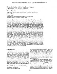
Figure 2. The (a) mixture-fraction pdf, fξg , is shown with (b) the conditionally averaged soot mass fraction, Qs . Heights are 0.9 (dashes) 1.4 (solid) and 1.9 (dash-dot) source widths.
the redistribution of energy through radiative transport. Both emission and absorption of soot are considered while gas-phase contributions are neglected. Because of the nature of the simulation with only one line of the domain available at an instant, an averaged radiation field was computed based on the soot and temperature fields of the previous realizations of the simulation. This averaged radiation field couples to the ODT evolution through radiative absorption and emission source terms in the instantaneous enthalpy equation. Coupling the radiation solution in this manner enables the ODT evolution to proceed as a parabolic marching problem. In the ODT simulations reported here, a fire nominally 1 m in width at its base is simulated on a computational domain 5 m in width to a height of 7.5 m. The fuel is ethene supplied at a constant mass flux rate of 60 g/m2 /s to match typical fire heatrelease rates. An adaptive griding technique, based on gradients of mixture fraction and soot, is employed for efficiency. The smallest length scales resolved are ≈ 100 µm in width, which is approximately the smallest estimate for the soot dissipative scale (Corrsin scale), and the average vertical step size is less than 10 µm. The results are ensemble averaged over approximately 1000 realizations. Statistics are further spatially filtered to reduce statistical noise using box filters centered in the domain of a width 0.24 m and height 0.12 m; the scale of these filtering boxes is limited by enthalpy variations due to radiation in the transverse transverse and by the mixing of fξg in the vertical direction. The ODT domain is sampled twenty times per realization for each box, every 0.006 m. Conditional statistics are resolved to bins of width 0.01 in ξg .
4. Results In this section, the general characteristics of the simulation describing the soot evolution in fires is presented followed by an analysis of the terms in Eq. (2.14). The results of the ODT simulations are employed to conduct an a priori analysis to assess the significance of these terms and the quality of the proposed closures. It is noted that the ODT model provides a set of evolution equations for which the non-linear advection terms are represented by a model not in the same form as the Navier-Stokes. Care must�be taken in assessing these terms, here primarily represented by the term ∇· hρ~v ys0 |ηi fξg in Eq. (2.14). Further, it is important to maintain consistency by using the ODT-determined values for both fξg and χ. Results are presented here only in the vicinity of the centerline and one to two source widths above the source. Earlier in the evolution the turbulence
318
J. C. Hewson et al.
is still developing, and later in the evolution the majority of the rich regions have been mixed out so that the results are less interesting. In Fig. 2, the mixture-fraction pdf and the soot mass fraction are shown for three heights above the source. As the flow evolves (moving up from the source), the mixture is observed to become leaner as rich pockets are mixed out. Simultaneously, the soot mass fraction just to the rich side of the flame (ξg ≈ 0.1 to 0.15 compared to a stoichiometric value of 0.06) increases. The evolution of the soot is in qualitative agreement with the observed evolution of soot over the scale of the fire (not shown) except that in the ODT simulation the results are resolved in the mixture-fraction coordinate; resolution of scalars with respect to the mixture fraction is beyond current experimental capabilities in sooting environments. The observed evolution is a consequence of the relatively slow soot chemistry, the radiative heat losses and the various means of soot transport in mixture-fraction space. The focus here is on modeling the latter. Before discussing the different means of soot transport in detail, the diffusion coefficients appearing in Eq. (2.4) provide some immediate guidance as to the importance of certain terms. In the second and third terms of Eq. (2.4) the soot diffusivity appears, implying that these terms are reduced by a factor of 1/Les relative to the fourth term in which the mixture-fraction diffusivity also appears. These terms are transformed by Eq. (2.6) into the second term on the r.h.s. of Eq. (2.14). For near-unity Lewis-number species, this term is often of primary importance for transport relative to the mixture fraction, but the opposite is true here because of the large magnitude of Les . These same terms in Eq. (2.4), through the use of Eq. (2.6), lead to the residual correlations, RDS and RCD , in Eqs. (2.10) and (2.11) that have generally been neglected in first-order CMC. In fact, these terms are the same magnitude as the second term on the r.h.s. of Eq. (2.14), but RDS and RCD tend to balance each other. This implies that even in the presence of differential diffusion where the closure hypothesis presented in Eq. (2.6) results in substantial residuals, the net effect is relatively small errors as suggested by Klimenko and Bilger (1999). Because all of these terms are inversely proportional to Les , all of these contributions are relatively small in the present case. Similarly small are the thermophoretic contributions and the diffusion of the pdf, the last three terms in Eqs. (2.4) and (2.14). The major contributions to the evolution of Ys in Eq. (2.4) come from the differential diffusion of soot and the mixture fraction (fourth term on r.h.s.) and the soot source terms (first and fifth terms on r.h.s.) as well as the vertical advective flux (left-hand side or l.h.s). Through Eqs. (2.7) and (2.12) and the application of the chain rule, the differential-diffusion term is split into the third and fourth terms on the r.h.s. of Eq. (2.14) as well as RDD . Each of these terms is plotted in Fig. 3 for two averaging boxes (1.4 and 1.9 source widths) and discussed in the following. The significance of these locations is that they represent a transition in the location of the pdf from being centered on the soot-production region to being centered on the soot-oxidation region. The differential-diffusion term in Eq. (2.4) is important because the mixture fraction, and thus the flame, diffuses more rapidly than the soot itself. This diffusive motion of the flame past soot leads to the most substantial diffusion-driven transport in mixturefraction space. This is split into three terms on the r.h.s. of Eq. (2.14). The first involves ∂ 2 (ρη χη fξg )/∂η 2 that is understood from the equation for fξg to be related to the evolution of fξg through terms like ∇ · (hρ~v |ηi fξg ) that also appear on the l.h.s. if the chain rule is applied to the advective scalar flux term. This partially offsets the advective scalar flux since a large part of the flux is associated with the evolution of fξg .
CMC with differential diffusion for soot 1 significant terms in Eq. 2.14
significant terms in Eq. 2.14
2 1.5 1 0.5 0 −0.5 −1 0
319
0.05
0.1
η
0.15
0.2
0.25
0.5 0 −0.5 −1 −1.5 0
0.05
η
0.1
0.15
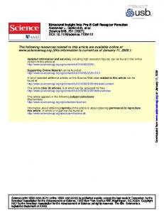
Figure 3. The significant terms in Eq. (2.14) are shown for a height of 1.4 source widths (left) and 1.9 source widths (right). The dashed line is the vertical advective flux; the dash-dot line is the flux of fξg (r.h.s. term 3); the solid line with squares is the soot source term (r.h.s. term 1); the solid line with circles is the soot source term contribution to the mixture fraction evolution (r.h.s. term 5); the solid line with triangles is the differential diffusion due to the evolution of fξg (r.h.s. term 4); the solid line with diamonds is the differential diffusion due to fluctuations (RDD ).
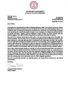
The second term involves ∂(ρη χη fξg )/∂η and ∂Qs /∂η. The first of these is a velocity in the mixture-fraction coordinate so that the combined term is a flux in the mixturefraction coordinate due to the contraction of fξg , referred to as the differential diffusion due to the evolution of fξg in Fig. 3. This has previously been recognized by Pitsch (1998) as being significant in transporting soot toward lean regions. At the height of 1.9 source widths where the mean ξg is approaching its stoichiometric value, this term increases in importance and is among the most significant in bringing the soot into the highest temperature regions. The residual associated with the approximation for the differential-diffusion terms in Eq. (2.7), RDD , is also of the same order of magnitude as the original term. Thus, all three of the residual correlations are of the same magnitude as the models for the original terms. Because RDD has Dξ in it, its significance is much greater than RDS and RCD and is discussed in greater detail here. In Fig. 4 the two sides of Eq. (2.7) are plotted along with their difference, which appears differentiated in Eq. (2.12). It is clear that the approximation provided in Eq. (2.7) is poor, especially in the important regions where soot is produced and oxidized and where the radiative source term is significant. In Fig. 3 it is seen that this poor approximation results in RDD that is of such a magnitude as to be one of the most significant sources in the CMC equation there. The approximation in Eq. (2.7) is equivalent to a presumption that ∇ · [(Dξ − Ds )∇ξg ] and Ys are independent, but Fig. 4 suggests that they are fairly well correlated. This correlation is explained by understanding that a negative value for ∇ · [(Dξ − Ds )∇ξg ] implies that the mixture fraction of a fluid element is getting leaner. It is reasonable to presume that a fluid element that was rich and is getting leaner will be associated with larger soot concentration (and vice versa), at least in the near-stoichiometric regions shown in Fig. 4. We have not measured the correlation coefficient, but the differences between Fig. 4 (a) and (b) suggest that this correlation coefficient may change through the fire. Because RDD is indicated to be a significant term in the transport of soot in mixturefraction space, it is desirable to identify a suitable model. A model is suggested by the
s ξ
(b)
ξ
−0.01 −0.02
s
s
ξ
−0.01
g
−0.02
−0.03
f
f
g
0
f
f
0
0.01
〈∇(D ρ∇ξ ) Y 〉 f and 〈∇(D ρ∇ξ )〉 Q f
(a)
g
〈∇(D ρ∇ξ ) Y 〉 f and 〈∇(D ρ∇ξ )〉 Q f
0.01
g
J. C. Hewson et al. s ξ
320
−0.03 0
0.05
0.1
η
0.15
0.2
−0.04 0
0.05
η
0.1
0.15
Figure 4. Terms involved in transport due to differential diffusion. The l.h.s. of Eq. (2.7) is shown in solid, the r.h.s. is the dashed line and the difference between the two is the dash-dot line. Heights are (a) 1.4 and (b) 1.9 source widths. 1 (a)
1 0 −1 −2 0
0.05
0.1
η
0.15
0.2
terms in Eq. 4.1
terms in Eq. 4.1
2
(b)
0.5 0 −0.5 −1 0
0.05
η
0.1
0.15
Figure 5. Proposed model for RDD . The l.h.s. of Eq. (4.1) is shown in solid, the r.h.s. is the dashed line. Heights are (a) 1.4 and (b) 1.9 source widths.
nature of ∇ · [(Dξ − Ds )∇ξg ]. This source of differential diffusion is strongest at the highest wave numbers and can be expected to be short lived and of random sign. In mixture-fraction space, this causes fluid elements to experience short-lived motions of random direction in η, suggesting a turbulent diffusion process. This would be modeled using the form of the second term on the r.h.s. of Eq. (2.14) so that we propose RDD ≈ −
ρ η χ η f ξg ∂ 2 Q s . 2LeDD,t ∂η 2
(4.1)
Introduced here is an effective turbulent Lewis number associated with diffusion in the mixture-fraction coordinate due to differential diffusion, LeDD,t . Setting LeDD,t = 1 the left and right side of Eq. (4.1) are plotted in Fig. 5. There is substantial noise in the evaluation of the second derivative, ∂ 2 Qs /∂η 2 , but the results indicate that the model for RDD proposed in Eq. (4.1) has the correct form. Further, the results indicate that LeDD,t is close to unity. This is particularly significant since it suggests that the model is consistent with the observations that a unity Lewis number works well for species subject to differential diffusion in turbulent flows. In addition, this model does not require the solution of an additional transport equation for every species subject to differential diffusion as proposed by Kronenburg and Bilger (1997). Also important in Fig. 3 are the two contributions of the soot source terms. These act together to produce the soot and to move it to leaner regions because the gas phase becomes leaner where carbon is transformed to soot (and vice versa). The source terms are
CMC with differential diffusion for soot
321
more significant lower in the flame where the dissipation rates are higher. The modeling of the coupled source with the scalar proposed in Eq. (2.8) is found to be accurate to within a few percent. Finally, the vertical flux of the soot is significant, showing the strong effect of the evolution over the entire fire �on the soot profiles in the ξg coordinate. The scalar flux fluctuations, ∇ · hρ~v ys0 |ηi fξg , are small, at least in the region where the results are presented here. This is surprising since both Kronenburg and Bilger (1997) and Nilsen and Kos´aly (1997) found that this term was important for moving the differentially diffusing scalars back toward the equal-mixing line. Because of the different derivation of the CMC equation employed here, it is possible that this effect is retained in a different term. Specifically, the residual correlation terms RDS , RCD and RDD do not appear in their derivations. Also, as noted by Kronenburg (1997), the evaluation of the scalar-flux fluctuations is challenging, and within the context of ODT it is even more so; this term requires additional analysis. In Sec. 2.1 it was suggested that employing a mixture-fraction equation with a soot source term was preferable in the present scenario. This deserves comment. If Eq. (2.2) was retained to define the evolution of ξ, the differential-diffusion term on the r.h.s. of Eq. (2.2) would result in a term in the CMC equation of similar form to the fourth term on the r.h.s. of Eq. (2.4), except that the soot gradients would appear and it is of opposite sign, −∇ · [ρ(Dξ − Ds )∇Ys ]. This term is found to be almost as large as, and of opposite sign to, the fourth term on the r.h.s. of Eq. (2.4); this indicates that the differential diffusion is not determined by ∇ · [ρ(Dξ − Ds )∇ξ] but by the difference between ∇ · [ρ(Dξ − Ds )∇ξ] and ∇ · [ρ(Dξ − Ds )∇Ys ], which just happens to be ∇ · [ρ(Dξ − Ds )∇ξg ] as appears in Eq. (2.4). Further, in every term where ∇ξ appears in any form (i.e., the scalar-dissipation rate as well as the differential-diffusion terms), the gradient would be composed of the combined gradients of ξg and Ys . With Les being large, the maximum values for ∇Ys are greater than those for ∇ξg , and the contribution of ∇Ys to all of these terms is significant. The result is that scalar-dissipation rates need to be known for the total mixture fraction, including the contribution from the soot, and also for just ξg to estimate the differential-diffusion terms from Eq. (2.13). Because the simple model suggested in Eq. (2.8) for the contribution of ws to the evolution of ξg works well, it is found that the use of the gas-phase mixture fraction results in an easier closure problem than the use of the total mixture fraction.
5. Conclusions The CMC equation for the evolution of soot was derived starting from the jointpdf equation for ξg and Ys and retaining residual terms associated with errors in the typical closure models. The resulting CMC equation is compared with the results of ODT simulations based on a new spatially evolving formulation. The terms involving differential diffusion are found to be important along with the soot source terms and the large-scale evolution of both the mixture fraction and the soot. Of particular importance in the regions of mixture-fraction space around the soot production and consumption is a residual term, not previously identified, that comprises the correlation between the differential diffusion and the soot mass fraction. This term results in a diffusion-like behavior in the mixture-fraction coordinate that has an apparent Lewis number near unity. The results here also suggest that when a large Lewis number component is a non-
322
J. C. Hewson et al.
negligible component of the mixture fraction, it may be easier to employ a mixture fraction, like ξg , neglecting this component. Such a mixture fraction variable has a source term that can be closed with the simplest of models.
Acknowledgments We are indebted to fellow summer program participants for their helpful suggestions, in particular to Luc Vervisch and Heinz Pitsch. Valuable discussions with Jay Gore throughout the development of the ODT models are appreciated. This work was conducted through support from Sandia National Laboratories, a multi-program laboratory operated by Sandia Corporation, a Lockheed Martin Company, for the United States Department of Energy’s National Nuclear Security Administration under Contract DEAC04-94AL85000. REFERENCES
Ashurst, W. T., Kerstein, A. R., Pickett, L. M. & Ghandhi, J. B. 2003 Passive scalar mixing in a spatially-developing shear layer: comparison of one-dimensional turbulence simulations to experimental results. Phys. Fluids 15, 579–582. Bilger, R. W. 1993 Conditional moment closure for turbulent reacting flow. Phys. Fluids A 5, 436. Echekki, T., Kerstein, A. R., Chen, J.-Y. & Dreeben, T. D. 2001 Computations of turbulent jet diffusion flames using the ‘one-dimensional turbulence’ model: Hydrogen-air flames. Combust. Flame 125, 1083–1105. Fairweather, M., Jones, W. P. & Lindstedt, R. P. 1992 Predictions of radiative transfer from a turbulent reacting jet in a cross-wind. Combust. Flame 89, 45–63. Hewson, J. C. & Kerstein, A. R. 2001 Stochastic simulation of transport and chemical kinetics in turbulent CO/H2 /N2 flames. Combust. Theory Model. 5, 669–697. Kerstein, A. R. 1991 Linear-eddy modeling of turbulent transport. Part 6. Microsstructure of diffusive scalar mixing fields. J. Fluid Mech. 231, 361–394. Kerstein, A. R. 1999 One-dimensional turbulence: Model formulation and application to homogeneous turbulence, shear flows, and buoyant stratified flows. J. Fluid Mech. 392, 277–334. Klimenko, A. Y. 1990 Multicomponent diffusion of various admixtures in turbulent flow. Fluid Dynamics 25, 327–333. Klimenko, A. Y. & Bilger, R. W. 1999 Conditional moment closure for turbulent combustion. Pro. Energy Combust. Sci. 25, 595–687. Kronenburg, A. & Bilger, R. W. 1997 Modelling of differential diffusion in nonpremixed nonreacting turbulent flows. Phys. Fluids 9, 1435–1447. Kronenburg, A., Bilger, R. W. & Kent, J. H. 2000 Modeling soot formation in turbulent methane-air jet diffusion flames. Combust. Flame 121, 24–40. ´ly, G. 1997 Differentially diffusing scalars in turbulence. Phys. Nilsen, V. & Kosa Fluids 9 (11), 3386–3397. Pitsch, H. 1998 Modellierung der z¨ undung und schadstoffbildung bei der dieselmotorischen verbrennung mit helfe interaktiven flamelet-modells. PhD thesis, RWTHAachen.
CMC with differential diffusion for soot
323
Pitsch, H., Chen, M. & Peters, N. 1998 Unsteady flamelet modeling of turbulent hydrogen/air diffusion flames. Proc. Comb. Inst. 27, 1057–1064. Pitsch, H. & Peters, N. 1998 A consistent flamelet formulation for non-premixed combustion considering differential diffusion effects. Combust. Flame 114, 26–40. Pitsch, H., Riesmeier, E. & Peters, N. 2000 Unsteady flamelet modeling of soot formation in turbulent diffusion flames. Combust. Sci. Tech. 158, 389–406.