Examples include the conditional simulation of geological variates of the Crystal. Viking petroleum reservoir, Alberta, Canada. KEY WORDS: Geostatistics ...
Mathematical Geology, Vol. 22, No. 3, 1990
Conditional Simulation of Intrinsic Random Functions of Order k I Roussos Dimitrakopoulos 2'3
Conditional simulation of intrinsic random functions of order k is a stochastic method that generates realizations which mimic the spatial fluctuation of nonstationary phenomena, reproduce their generalized covariance and honor the available data at sampled locations. The technique proposed here requires the following steps: (i) on-line simulation of Wiener-Levy processes and of their integrations; (ii) use of the turning-bands method to generate realizations in Rn; (iii) conditioning to available data; and (iv) verification of the reproduced generalized covariance using generalized variograms. The applicational aspects of the technique are demonstrated in two and three dimensions. Examples include the conditional simulation of geological variates of the Crystal Viking petroleum reservoir, Alberta, Canada.
Geostatistics,nonstationaryphenomenon, Wiener-Levyprocess, stochasticsimulation, generalized covariance, generalized variogram. KEY WORDS:
INTRODUCTION Conditional simulation of stationary natural processes was introduced in geostatistics by Journel (1974). Several aspects and developments on stationary simulations have recently been presented (Christakos, 1987; Davis, 1987; Mantoglou, 1987; Luster, 1985). Conditional simulation of nonstationary stochastic fields has seldom been addressed apart from the first use of the method in two dimensions (Chiles, 1977) and two early applications (Delfiner and Chiles, 1977; Delfiner and Delhomme, 1973), despite the fact that geological variables commonly exhibit distinct trends. Such variables are properties of petroleum reservoirs like porosity, fluid saturations, boundaries, etc. (Dimitrakopoulos, 1988). As in the stationary case, conditional simulations of nonstationary fields which mimic the spatial variability of the actual phenomenon under study can ~Received 12 July 1988; accepted 15 September 1989. ZD6partement de G6nie Min6ral, l~cole Polytechnique, C.P. 6079 - Succursale "A," Montr6al, Qudbec, H3C 3A7, Canada. 3present address: Departmentof Mining and Metallurgical Engineering, McGill University, 3480 University Str., Montr6al, P.Q., Canada H3A 2A7. 361 0882~g 121/90/0400-0361 $06.00/1 © 1990 International Association for Mathematical Geology
Dimitrakopoulos
362
be generated. The latter property is of particular interest in sensitivity studies. In the petroleum industry, for example, it is fundamental to assess the sensitivity of reservoir-flow simulations to possible variations of the geological input. This can be done objectively by using realistic representations of the fluctuation of the pertinent variables as provided by conditional simulations. In the present study, a comprehensive step-by-step procedure of conditional simulation of nonstationary physical processes is developed, within the framework of the theory of intrinsic random functions of order k and the turning-bands method (Matheron, 1973). More specifically, the procedure includes the following steps. First, the Wiener-Levy process is used to simulate an IRF-k in R ~. Then, simulations in R n are obtained by summing contributions from those in R ~. The conditioning process is described and the quality of the simulations is examined using experimentally calculated generalized variograms. In order to gain some insight into practical aspects of the proposed technique, examples in two and three dimensions are given. NONCONDITIONAL SIMULATIONS
The Wiener-Levy Process A Wiener-Levy or Brownian motion process is a stochastic process { W ( x ) , x -> 0 } in R 1 with the following properties (Parzen, 1962; Antelman and Savage, 1965) i. { W ( x ) , x _> 0 } has stationary independent increments. ii. For all x > 0: W ( x ) is normally distributed. iii. For allx > 0: E [ W ( x ) ] iv. W(0) = 0.
= O.
As a consequence of (i) and (iv), to state the probability law of W ( x ) , it is sufficient to state the probability law of [ W ( x + h) - W(x)] with x + h > x. Because of (ii), the increment [ W ( x + h) - W(x)] is normal and its law is determined by its mean and variance. It is E [ W ( x + h / - W(x/] = 0
(1)
and Var[W(x + h) - W(x)] = a 2
Ihl
(2)
where a 2 is a characteristic of the process in hand. In addition, one may consider the pth integration Wp (x) of a Wo (x) process in R ~ such that
wp(x) :
f
x(x
_ .yo-,
o (p :--
Wo(.) d . ,
P = 0,
k . . . .
(3)
Conditional Simulation of Intrinsic Random Functions of Order k
363
The discrete Wiener-Levy process Wo(x ) is defined as an IRF-0 (Orfeuil, t972) by the relation (iv) and v. F o r a l l i e [1 . . . . .
n]: Wo(xi) = W o ( x i - 1 ) + Ri.
vi. For all x ~ [x i, xi + 1]: Wo (x) = W o (xi). Here { Ri, i = 1 . . . . . M } is a set of independent random variables with realizations of values + 1 or - 1 and probability of occurrence 1 / 2 . Note that relations (i) and (iii) remain valid in the discrete case. Relation (ii) holds if R i follows a Gaussian law. The discrete process Wp (x) may, in addition, be defined by vii. Wp(O) = 0 f o r a l l p >_ 1. VIII.
Wp(xi) = We(xi_ 1) + e w e - l(xi), for allp > 1 where e is the norm of vector F = XoX 1 XiXi + 1" =
ix. For all x 6 [xi, x i + l ) : Wp(x) = Wp(xi). Note that relations (viii) and (ix) are not verified by Eq. (3). For the discrete process Wo(x), it is easy to show that Eq. (1) is valid, as each R i has zero expectation. In addition, it is Var[Wo(x + h ) = E
L\p=i+l
Wo(x)] = E [ ( W o ( x + h) - Wo(x)) 2] Re
)21
= (j - i)
E[R21
where R = Re, for all p, and i and j are defined by
x + h ~ [x;, x j + , ) j>i Setting ( j - i ) e = [h I, one obtains m
Var[Wo(x + h) - Wo(x)] = --]hiE [R 2] e
which becomes
Var [Wo(x + h) - Wo(x)] = il i h l Since Var [Wo(x + h) - Wo(x)] = - 2 K o ( h )
(4)
364
Dimitrakopoulos
Equation (3) shows that the generalized covariance (GC) o f Wo(x ) will be 1
K°(h) = -2e
Iht
(5)
In conclusion, one can construct a realization of a Wiener-Levy process W o ( x ) in R 1 by simply generating random numbers of + 1 or - 1 drawn with equiprobability, and by applying properties (v) and (vi). The produced realization will have a GC K ( h ) = - I h l (Fig. 1). From this, realizations of the pth summation o f Wo (x) can be generated. Simulation of I R F - k in R 1
It has been shown (Matheron, 1973) that an IRF-k in R l admits a polynomial generalized covariance (GC) if and only if it admits the representation
~(x) : boWo(x) + b,
S"
o Wo(u) d . + . . .
S
+ bk o - ( £ - - ~ .
Wo(u)d. (6)
with bp real coefficients, and W o ( x ) a representation of an IRF-0 with a GC such that K ( h ) = - [h [.
E x peri mental points . . . . . : •
12
Average ofl5
lines
/ •
--
iO
f, 4-
0 0
I I
I 2
I 3
I 4.
I 5
I 6
DISTANCE
I 7
I 8
I 9
I I0
I II
I 12
13
(hi ~
Fig. 1. Experimental and theoretical variograms of realizations of Wiener-Levy processes on lines with k(h) = - Ih I.
Conditional Simulation of Intrinsic Random Functions of Order k
365
Equation (6) may be rewritten as
k
Y(x) : Z % % ( x )
(7)
p=O
Wp(x) is defined in Eq. (3). Wp(x) is an IRF-p with a GC-p
where
ihl2P+l
(--1) p+t
Ke(h) - (2p + 1)!
,
p = 0 .....
k
(8)
Note that since Wp(x) is an IRF-p it is also an IRF-k for a l l p _< k. If Y(x) is an IRF-k in R l , which admits the representation (6) or its equivalent (7), and the linear combination
E xov(xo)
a=l
is a GI-k, then
XaY(Xa
Var
= 2
a=l
2 X~XbK1(& - xh)
a=l
(9)
b=l
where K1 (h), h = x~ - xo, is the GC-k of Y(x). In addition, taking Eq. (7) into account, one finds
XY(xa
Var
2 Xa 2 bpWp(x)
= Var
a=l
La=l
= a2 , O~' X~Xb =
=
~]
2
bpbqE(W,(xa) Wq(xb)
•
bpbq Kp' q(Xa - Xb)
q=O
p=O
= a21 b21 )ka)kb p =•0 = =
p=O
q=O
([O)
where Kp,q(h) is the cross GC of the IRF-k's Wp(x) and Wq(x). Given that the derivatives of Wp(x) and Wq(x) defined by Eq. (3) are W(pP)(x) = Wo(x) and W(qq)(x) = Wo(x), respectively, f o r p , q = 0 . . . . , k, the cross GC Kp,q(h) is such that
d p +q
dhP+q X,,,q(h) = ( - 1 < Ko(h) where for Ko (h) = - co I h I concludes
Kpq(h) : ( - 1 ) p+~ '
co (p + q + 1)!
ihlp+q+i
(11)
366
Dimitrakopoulos
It follows from Eqs. (9) and (10) that the GC of Y(x) is
Kl(h ) =
k
k
~]
~] bpbqKp,q(h)
p=0 q=0 k
k-I
= Z b2Kp,p(h) + 2 Z
q=Op>q
p=O
bqbpgp, q(h)
(12)
Equations (11) and (12) give k
60
K,(h) = N a p ( - l ) p + ' (2p + 1)! ]h p=O
[2p+l
(13)
with a; = (-1) p+I (bp) 2 ÷
p-1 Z
( - - 1 ) i+1 2bib2p_ ,
(14)
i=max(O,2p-k)
From Eqs. (13) and (14), Table 1 may be constructed showing the representation of an IRF-k in terms of Wiener-Levy processes and corresponding GC in R 1 for k < 2. It follows from the above that realizations of an IRF-k in R ~ with given polynomial GC with real coefficients can be generated from realizations of the processes Wo(x) and Wp (x), provided that the appropriate coefficients are calculated. For example, if k = 2 and the required GC in R I is
K,(h)
=
-aolh[ + ~a ' l h l 3 _ a 2 l h [ 5
it is sufficient to simulate a realization of the IRF-2
Y(x) : boWo(x) + b,w,(x) + b2W2(x) Table 1. Representation of an IRF-k in Terms of Wiener-Levy Processes and Corresponding GC in R ~for order k < 2 k
Y(x)
0
boWo(x)
1
boWo(x) + b, W, (x) boWo(x) + b, W,(x) + b2W2(x)
K,(h)
-bo~O,lhl -bo~,,,Ihl + bye. Ihl 3 ¢d [hi 3 -- b~2 ~.. O) [h[5 - b ~ l h [ + [b~ - 2bobz] ~..
Conditional Simulation of Intrinsic Random Functions of Order k
367
where the coefficients are calculated by solving the system b 2 = ao b 2 - 2bob2 = al b22 = a2 What needs to be shown next is how from simulations of an IRF-k in R ~, realizations in R" can be constructed, and what the relations between the coefficients of the one-dimensional and n-dimensional GCs must be in order for the n-dimensional realization to have a specific GC.
The Turning-Bands Method and Simulation of IRF-k in R" It has been shown (Matheron, 1973) that if Y ( x ) is an IRF-k in R ~ with GC KI (h), an IRF-k in R" is defined such that
(15)
z,(x) = Y((x. , ) )
where Y is the projection of vector x on s (Fig. 2), s is a unit vector chosen randomly from a unit sphere in R" with probability ~n concentrated in the sphere and invariant under translation. Then, Z s ( x ) has an isotropic GC such that r Kn(h) = ~ Kl((h
• s})~nds
(16)
Equation (16) defines a one-to-one mapping of the GC-k in R 1 to an isotropic GC-k in R ~, and it is called the turning-bands operator (Tn). For the operator T,, the equivalent GCs in R 1 and R" are, respectively, the following
k
]hl2P +I
K l ( h ) = ~] ( - 1 ) p+l ap p=O
(2p + 1
)!
(17)
and
l h] >+~ /¢~(h) = p=o Z ( - 1 ) p+' apB.,p (2p + 1)r with B,,,p = p! r'
(2)( (!+n)) 7r1/2 I'
P +
2
(18)
Dimitrakopoulos
368
Si
x.sj F i g . 2. S c h e m a t i c representation o f the t u r n i n g - b a n d s operator.
It follows that if a random field having a polynomial GC with coefficients, say Cp, is to be simulated in R ", the coefficients ap of the GC in Eq. (17) are
Cp
(19)
ap = On,p From Eq. (19) it follows, for example, that in R 2 and for k = 2, 71" ao
=
97r at = T C I (15)2~r a2 -- _
_
2
C2
Finally, if the appropriate random fields in R ~ can be simulated, then an n-dimensional field can be constructed by applying 1
N
Zs~v(x) - N,/2 i~ 1 Yi( (x " Si) )
(20)
which is the discrete approximation of Eq. (15), with N being the number of independent one-dimensional random fields (Fig. 2).
C O N D I T I O N A L S I M U L A T I O N OF R A N D O M FIELDS W I T H GENERALIZED COVARIANCES Conditional simulation of an IRF-k Z(x) in R n is a technique which, given values of Z(x) at particular points {xa, a = 1 . . . . . N} and the corresponding
Conditional Simulation of Intrinsic Random Functions of Order k
GC, allows the construction of different realizations of following two properties:
369
Z(x), which have the
(i) honor the given data available at { x a, a = 1 . . . . (ii) reproduce the GC of Z ( x ) . it.
, N };
Consider an IRF-k S(x) with the same GC as Z ( x ) but not correlated to S(x) can be simulated as previously shown. One can write
S(x) = S * ( x ) + [S(x) - S * ( x ) ] The conditional simulation of then defined as
Z(x), {xa, a = 1, . . . , N} with GC K(h) is
Zc,(X) = Z*(x) + [S(x) - S * ( x ) ]
(21)
where S*(x) is estimated (kriged) as if S(x) is only known at points {xa}. Apparently, Zc, (x) will reproduce the data { x~ } because Z * (x~) = Z (x a) and S(xa) = S* (xa), which follows from the exactness of the kriging estimator. Consider now the covariance between the kriging error and all increments of order k. It has been shown (Delfiner, 1976) that they are orthogonal to each other
E
Coy Z(xo) - Z*(xo),
m xbz(x~ ,i = o
Z
b=l
Zcs(X) at any point Xb, one finds
By taking a k th increment of
m
~=, XbZcs(X~) = Z
m x~z*(xO +
b=l
Z
x~(s(~)
- s*(x~))
b=l
then it is Var
Xb s b
1
Xb
= Var
XbZ* xb
I
b=l
_
+ Var
Xb(S(xb) -- S*(Xb b
Since
I
Z(x) and S(x) have the same GC, then Var[b~,
XbZcs(Xb)? = V a r [ b ~ , XbZ(Xb)1
The above shows that indeed Zcs(X) and Z ( x ) have the same generalized covariance. Furthermore, one can show that the estimation variance of Zcs(X) is
370
Dimitrakopoulos
twice the estimation variance of Z* (x). Indeed
e[(z(x)
- Zcs(X)) 2]
: e[(z(~)
- z,(~)
-(s(~)
= e[(z(~)
- z,(~)) ~ + (s(x) - s,(~)) ~
- 2(z(~) - z,(~))(s(~)
= e[(Z(x) =
- s , ( ~ ) ) ) ~]
- s,(x))]
- z , ( ~ ) ) ~] + e [ ( s ( ~ )
2E[(Z(x)
- s , ( ~ ) ) 2]
Z*(x)] 2]
-
(22)
VERIFICATION OF SIMULATIONS USING GENERALIZED VARIOGRAMS
The reproduction of a given generalized covariance of a conditionally or nonconditionally simulated realization of an IRF-k may be checked by comparing the experimental and theoretical generalized variograms (GV) in different directions. GVs are simpler to obtain but directly related to GCs. Aspects of the GV related to the present subject are presented next. Additional information may be found elsewhere (Christakos, 1984; Chiles, 1979). The generalized variogram of order k is 1
7k(h) - ,-.k+l Var [Ak(x, h)]
(23)
V'2k + 2
where Ak(x, h) is a generalized increment of order k (GI-k) such that k+l
Ak(x,h) = ~
( - 1 ) iCk+i , r ( x + ih)
(24)
i=0
whereCK+i i = (~ +l). Note that, the GI-k in Eq. (24) is stationary if Y(x) is an IRF-k, and therefore -/k(h) in expression (23) is independent ofx. In addition, it is Var[k~(x, h)] = E[(Ak(x, h)) 2] k+l
k+l
= Y] ~], (--1)i+Jcik+, C ~ + , K ( ( i - j ) h ) j=O
i=0 k-I =
E l= --k- 1
( - 1 ) ' ~t-t+k+, ' 2 ( k + 1) K(lh)
Conditional Simulation of Intrinsic Random Functions of Order k
371
and therefore k+l
1 3'k(h) - ,.~k+l
Z
( _ 1 ) t ,~2¢k+1) ,.~k+ 1 +,
"-'2k + 2 [ = - ( k +
K(lh)
(25)
1)
From Eq. (25), the relations between generalized covariances and generalized variograms for k = 0, 1, 2 in R 1 may be derived. More specifically, it is
% ( h ) = K(O) - K ( h ) "yl(h) = K ( 0 ) - 4 / 3 K ( h ) + 1 / 3 e ( 2 h ) ~/2(h) = K ( 0 ) - 3 / 2 K(h) + 3 / 5 K(2h) - 1/10 X(3h)
(26)
The experimental generalized variogram may be calculated from 1
N~
yff(h) -
[ "2(k+
xk(x,
(27)
l)lVh i =
where N h is the number of finite differences A(x, h) available (e.g., the number of pairs Y(x + h) - Y(x) if k = 0). From Eqs. (27) and (24) it follows that fork=0, 1,2itis 1
Nh
"~ -- 2Nh i~=t [Y(x) - Y(x + h)] 2 1
uh
7* = 6N h i~=~ [Y(x) - 2Y(x + h) + Y(x + 2h)] 2
1
Nh
Y~ - 20Nh i~=' [Y(x) - 3Y(x + h) + 3 r ( x + 2h) + Y(x + 3h)] 2 (28) Concluding, Eq. (28) shows how the experimental generalized variograms of a realization of an IRF-k can be calculated for the common cases of k = 0, 1, 2 in one direction. Then it can be compared to the theoretical examples given by Eq. (26) to verify the reproduction of the GV.
TWO-
AND T H R E E - D I M E N S I O N A L E X A M P L E S
Realizations of an IRF-2 with generalized covariance
K(h) -- - I h l
+ 0.1 th[ 3 - 0.001 lhl 5
have been simulated in two and three dimensions. The two-dimensional realization (Fig. 3) is on a 40 × 40 regular grid of 1600 points and has been
372
Dimitrakopoulos
N X
Xl H
: I
grid spacing
F i g . 3. C o n t o u r m a p o f a nonconditional simulation o f an I R F - 2 in two dimensions.
constructed using 90 equi-angular one-dimensional simulations. The three-dimensional realization is on a 20 x 20 x 20 regular grid of 8000 points. It has been produced by summing 15 simulations on lines joining the midpoints of the opposite edges of a regular icosahedron, as is the standard practice (Guibal, 1972). A horizontal section from the middle of the generated grid is presented in Fig. 4. The reproduction of the GC was tested by calculating directional experimental generalized variograms and comparing them to the theoretical one. In the two-dimensional example, experimental GVs of order 2 were calculated along axes x, y, and the two diagonals. The comparison to the theoretical one is shown in Fig. 5. In the three-dimensional case, experimental GVs of order 2 were calculated along the three orthogonal axes and compared to the theoretical one in Fig. 6. Both comparisons suggest that the initial generalized variogram has been preserved reasonably well. The observed differences between simulated and theoretical values should be attributed to the discretization involved in the one-dimensional simulations, the finite number of lines used, and the normal statistical fluctuations. A detailed presentation of small biases introduced by the use of the discrete integrations of the Wiener-Levy processes can be found in Chiles (1977).
Conditional Simulation of Intrinsic Random Functions of O r d e r k
xl
373
---~
I---I : I grid spacing Fig. 4. Cross section from a nonconditionally simulated realization of an IRF-2 in three dimensions.
The conditional simulation of IRF-k is next applied to "real life" data from the Crystal Viking oil field, Alberta (Reinson et al., 1987). The first application involves elevations in meters below the mean sea level of the bottom of the Crystal Field using data from 144 wells. The GC inferred from the data set is of order 1 and has the form
K(h) =
- 0 . 0 2 7 6 9 1 !h[ + 0.000344 ]hi 3
A realization of the bottom of the Crystal Field (Fig. 7) was simulated on a grid of 38 x 50 points with a grid spacing of 300 meters. The reproduction of the GC is verified using the four one-dimensional GVs shown in Fig. 8. The second application includes the generation of a realization of percent porosity from a sedimentary unit within the Crystal reservoir. Available data include 186 regularized samples of 1 meter length, representing porosity derived from core analyses. The GC inferred from the data is of order 0 and geometrically anisotropic in two dimensions with Khor(h ) = 0.52 x 10 -3 - 0.666 x 10 - 6 ] h i Kve.(h) = 0.52 x 10 -3 - 0.121 x 10 -3
lh I
374
Dimitrakopoulos Experimental points
Direction
o o
Oo 45 ° 90 ° 135 °
70
60
50
t
°'/o
40
gO
l--I c-
30
~d >o 20
!0
O
!
2
3
4
5
6
DISTANCE
7
8
9
I0
II
h
Fig. 5. Experimental and theoretical generalized variograms of a simulated realization of an IRF-2 in two dimensions.
A realization of porosity was conditionally simulated on a regular grid of 19 × 32 × 105 points with a resolution of 300 meters horizontally and 1 meter vertically. The geometric anisotropy was treated by properly scaling the grid. A horizontal section and a cross section from a generated realization of porosity are presented in Figs. 9 and 10, respectively. The quality and reproduction of the GC is checked by computing experimental GVs of order zero on the horizontal and vertical planes. The results are plotted in Figs. 11 and 12, respectively, and show that preservation of the GC is excellent. S U M M A R Y AND C O N C L U S I O N S
A comprehensive step-by-step technique for the conditional simulation of IRF-k has been presented. The turning-bands operator transforms the problem
Conditional Simulation of Intrinsic R a n d o m Functions of O r d e r k
375
Experimental points
70-
Axis
D
X
0
Y
'~
Z
60" Theoreticai~
50-
t
r~
i O
40-
~0
&
D
30)~ 20-
I0
0 0
~ "ff I
~ "r 2
I 3
I 4
I
5
I 6
DISTANCE
I 7
I 8
I 9
I
IO
h
Fig. 6. Experimental and theoretical generalized vafiograms of a simulated realization of an IRF-2 in three dimensions.
of simulating n-dimensional random fields into simulation in R ~. On-line realizations of an IRF-k are generated using Wiener-Levy processes and their summations. The calculation of the appropriate coefficients for the processes on lines, so that they reproduce the GC of the IRF-k in R ~, is of main importance here. Next, by a folding-back procedure, realizations of IRF-k in Rn are constructed. Given the nonconditional simulations, conditional simulation of an IRF-k may be defined as the sum of an estimated random function using the IRF-k theory and a correlated variate with the same GC as the process under study. Conditional simulations of random fields honor the data values available and reproduce the GC of the physical process. Verification of the latter is performed in this study by using generalized variograms. The examples presented show that the conditional simulation of IRF-k is
376
Dimitrakopoulos
Fig. 7. Contour map of a conditionally simulated realization of the bottom of the Crystal Viking reservoir, Alberta, Canada.
Conditional Simulation of Intrinsic Random Functions of Order k
377
Experimental points
Direction
800
I
700
• Q
4,5 ° 90 o
0 °
0
135 °
OQ
GOD I
500
o
®
400 •
Q
300 200 IO0 0 0
t
I
I
300
600
900
I
I
1200
I
1500
DISTANCE
h
1800
I I 2:100 2400
I
2700
--T'-3000
(m)
Fig. 8. Experimental and theoretical generalized variograms of the realization of the bottom of the Crystal Viking reservoir, Alberta, Canada, as in Fig. 7.
C.D ,..3
co., .,5
,..__~:
i'~ s0 : ~"~ ~
.----. . . . .
Fig. 9. Horizontal section from a three-dimensional conditionally simulated realization of porosity of a sedimentary unit within the Crystal Viking reservoir, Alberta, Canada.
l
~. Conditionally simuloted boundary
J
~ i?°-
'----~,. ~ /
.~
.:L - . . D ~-~,
378
Dimitrakopouios
L.__
. . ~_~f
.~
t