Confidence Intervals for Reliability and Quantile ... - IEEE Xplore

IEEE TRANSACTIONS ON RELIABILITY, VOL. 55, NO. 4, DECEMBER 2006

591

Confidence Intervals for Reliability and Quantile Functions With Application to NASA Space Flight Data Astrid Heard and Marianna Pensky

NOTATION probability function i.i.d sample of a random variable cdf of at quantile function of at confidence coefficient

Abstract—This paper considers the construction of confidence intervals for a cumulative distribution function ( ), and its in1 ( ), at some fixed points , and verse quantile function on the basis of an i.i.d. sample = is rel=1 , where atively small. The sample is modeled as having a flexible, generalized gamma distribution with all three parameters being unknown. Hence, the technique can be considered as an alternative to nonparametric confidence intervals, when is a continuous random variable. The confidence intervals are constructed on the basis of Jeffreys noninformative prior. Performance of the resulting confidence intervals is studied via Monte Carlo simulations, and compared to the performance of nonparametric confidence intervals based on binomial proportion. It is demonstrated that the confidence intervals are robust; when data comes from Poisson or geometric distributions, confidence intervals based on a generalized gamma distribution outperform nonparametric confidence intervals. The theory is applied to the assessment of the reliability of the Pad Hypergol Servicing System of the Shuttle Orbiter.

—parameters of a generalized gamma distribution Fisher information matrix polygamma function

gamma function

Index Terms—Confidence intervals, generalized gamma distribution, Jeffreys non-informative prior.

inverse for

:

ACRONYMS1 KSC NASA PRACA PR

Kennedy Space Center National Aeronautics and Space Administration Problem Reporting And Corrective Action Problem Report

PHSS MLE HPD pdf cdf NPJef

Pad Hypergol Servicing System Maximum Likelihood Estimator Highest Posterior Density probability density function cumulative distribution function NonParametric confidence intervals based on Jeffreys prior NonParametric Second Order corrected interval Confidence intervals based on Generalized Gamma distribution

NPSO GenGam

Manuscript received September 19, 2005; revised April 29, 2006. This work was supported in part by the National Science Foundation (NSF) under Grant No. DMS-0505133. Associate Editor: R. H. Yeh. A. Heard, retired, is with NASA, USA. M. Pensky is with the Department of Mathematics, University of Central Florida, Orlando, FL 32816 USA. Digital Object Identifier 10.1109/TR.2006.884590 1The

singular and the plural of an acronym are always spelled the same.

posterior pdf of posterior pdf of

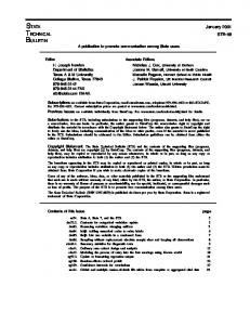
I. INTRODUCTION T the Kennedy Space Center (KSC), and other National Aeronautics and Space Administration (NASA) Space Flight Operations centers, a great deal of effort is expended to collect, analyse, and report statistical data on performance of space vehicle systems during tests, and operations. In all cases, an effort is made to mitigate the risk of failure, and improve safety and reliability by finding systems that may benefit from some sort of corrective action. Statistical data summarizing the performance of space vehicle systems can sometimes enable evaluation of the best possible type of corrective action to use, such as replacement versus redesign. Ultimately, the final decision for vehicle launch is subjectively based on the hope that all possible actions have been taken to ensure systems continue to operate safely and reliably. Fig. 1 is a representative plot of problem report counts for the Space Shuttle Orbiter Digital Processing System for a three month time period. Similar plots for all major Space Shuttle subsystems are produced periodically, and used to determine the existence of adverse trends requiring additional investigation.

A

0018-9529/$20.00 © 2006 IEEE

592

IEEE TRANSACTIONS ON RELIABILITY, VOL. 55, NO. 4, DECEMBER 2006

Fig. 1. Orbiter digital processing system problem reports.

The current practice of evaluation of various space vehicle systems relies heavily on the visual examination of data, usually represented in histogram form. Sometimes the data are evaluated based on the relationship of the data to the “goal” value, i.e. whether or not the data points exceeded (or remained below) this value. The above examination currently has one objective, namely the assessment of the presence of an unfavorable time trend in data for evaluation of whether the system under scrutiny is to be considered acceptable or sufficiently reliable to accomplish a space mission or some other pre-defined objective. However, it is clear that the absence of trend does not guarantee system safety. It is possible that a system under consideration is unacceptable, even prior to the current period of examination, but did not “fail,” as indicated by data, due to the stochastic nature of the situation. Therefore, it is vital to assess the reliability of parts and systems of space vehicles even if a time trend is absent. Initially, data can be examined to establish the presence of a trend (see e.g. [17]). However, in many situations, as in the example with the dice, a time trend is not present due to the identical distribution of the outcomes of the rolls. In much the same way, the problem counts (failures) derived from the NASA/KSC Space Shuttle Problem Reporting And Corrective Action (PRACA) database are very often trend free, and, for this reason, are not examined from a reliability point of view under the present system. The goal of this paper is to study trend-free data from the point of view of reliability. To draw a data-driven automatic decision, program managers usually want information on what is the probability that the number of problem counts of a certain system does not exceed a given threshold (say, ), and the proconfident in the results. gram manager wants to be, say, This, in fact, is a very common problem because the probability

that a random variable of interest, , does not exceed a cer, the distribution tain pre-specified value , function of variable at the point , is the main object of inference in many practical applications. For example, if is the life is just the probability time of a device under scrutiny, that this device will function for a longer time than . If is the number of failures of a certain piece of equipment within a is the probability that the number fixed time period, then of failures within a given time period is not more than , and so on. In practice, however, a point estimator of makes little may vary from its estisense because the actual value of mator quite significantly if the variance of the estimator is high. As a consequence, the information which decision making per, i.e. the value sonnel really want is a lower bound on such that, say, . Sometimes, there is a need to solve the inverse problem, namely, for a given proba. The bility find a number such that former can be re-written as , where is the quantile function of at the point . In more precise terms, these problems can be formulated as be i.i.d. samples of a random varifollows. Let able where the values represent the number or frequencies of occurrences of some events (e.g. failures of a system) within given increments of time. Let this sample have an unknown density function , and cumulative distribution function . Let be the quantile function of . The questions above can be posed as: (Q1) Given i.i.d. samples of a random variable , and and , find the values such that

(1)

HEARD AND PENSKY: CONFIDENCE INTERVALS FOR RELIABILITY AND QUANTILE FUNCTIONS

(Q2) Given i.i.d. samples of a random variable , find the values , that

, and such (2)

Observe that (Q1) is the problem of constructing the lower confidence bound for the distribution function at the known point , while (Q2) is equivalent to the construction of at some point . the upper confidence bound for its inverse The first problem is common in guaranteed coverage tolerance prediction described in, for example, [3]. The main challenge here is the development of fully data-based techniques of the construction of confidence bounds (1) & (2), which are suitable . In addition, in reliafor small sample sizes bility, one is interested in “extreme” values of & , namely, the values of such that , or , where is small. Hence, the inference deals with the tails of the distribution , and is based on a very small number of observations. This circumstance rules out nonparametric approaches which cannot successfully deal with the tails of an unknown distribution for small sample sizes. Additionally, nonparametric approaches usually result in relatively long confidence intervals because they are always designed for the least favorable distribution fitting the data. Hence, we need to choose a class of distributions which are flexible enough, but can still be treated parametrically. The distribution families most commonly used to model the lifetimes are the Weibull, or gamma distributions. Because they have different functional forms, the practitioners either choose one of them arbitrarily, or test the hypothesis of which one agrees better with the observations (see e.g. [20]). After distinguishing between the two distributions, and matching the shape parameter to the data, the confidence intervals are con, and . To avoid making structed for the values of this choice, and designing completely data-driven confidence is drawn from the intervals, we assume that the sample generalized gamma distribution introduced by Stacy [18] with the probability density function (pdf) (3) The advantage of using (3) is that it can emulate a wide variety of curves so that the majority of the distributions used in reliability are particular cases of (3). Parameter defines how thin the tails of the distribution (3) are. Hence, by accommodating close to zero, we include distributions with relatively heavy tails, while large values of lead to distributions with very thin tails. It should be noted that, due to its flexibility, statistical inference for the generalized gamma distribution is rather tricky. For example, it is not uncommon even with sample sizes of two- to three-hundred observations that algorithms evaluating the Maximum Likelihood Estimator (MLE) of , , and fail to converge (see e.g. [13]). The way out of this difficulty is either using the rather unreliable method of moments estimators (see e.g. [19]), or assuming one or two parameters of the generalized gamma distribution to be known (see e.g. [4], [14], or [16]). In practice, however, parameters of distributions are never known, so they are estimated from the data, and then the estimators are

593

plugged into the expressions for the confidence intervals. If we were to adopt this approach in the present paper, this would reduce the complexity of the problem. However, this practice would make constructed confidence intervals unreliable, especially because the amount of data available is small. To construct data-driven solutions to the questions (Q1) & (Q2) based on small samples, we shall design Bayesian confidence intervals based on the non-informative Jeffreys prior (see e.g. [5]). In our approach, we shall treat all three parameters of the generalized gamma distribution as completely unknown just making an (quite insignificant) assumption that the shape parameter is bounded from above. The rest of the paper is organized as follows. In Section II, we give background information on nonparametric methods for construction of confidence intervals. Section III describes the Bayesian approach to construct confidence bounds (1) & (2). Section IV is reserved for a simulation comparison between these two methods. Section V studies the robustness of the proposed approach when the actual data come from a distribution other than the generalized gamma. Section VI considers applications of the theory to real data. Section VII concludes the paper with discussion. Finally, in the Appendix, we present the proof that the posterior pdf derived in Section III is a proper probability density. II. EXISTING NONPARAMETRIC METHODS Construction of a nonparametric lower confidence bound for at a known point is intimately related to the interval estimation of a binomial probability on the basis of i.i.d. obserwith vations. To see this, form a new i.i.d. sample where is the indicator of the set . Then are Bernoulli variables with , the has a binomial distribution with paramehence, ters and , and problem (Q1) reduces to the construction of the lower confidence bound for on the basis of . , and the interval estimator The point estimator of is is based on . The above problem has a long history, and extensive literature , coverage (see e.g. [2], [6]–[9], and [11]). Because , the textbook lower bound and (contributed to Wald) is based on the asymptotic -normality of statistics , and has the form where is the percentile of the -normal distribution. A modification of this bound (leading to a Wilson, or score interval) is the positive solution of the simple quadratic . equation The intervals listed above, however, do not have adequate coverage, especially when is close to zero or one (which are often the cases of interest in reliability). Brown et al. [7], [8], and Cai [9] studied the existing confidence intervals for in detail, evaluated various confidence intervals suggested in literature, and came up with solutions to the problem. Cai [9] resolutely recommends the one-sided Jeffreys, and second-order corrected intervals as an alternative to Wald and score intervals. The Jeffreys interval is the Highest Posterior Density (HPD) interval constructed by Bayesian inference with Jeffreys prior, which in this case is Beta(0.5, 0.5). It is of the form Beta

(4)

594

IEEE TRANSACTIONS ON RELIABILITY, VOL. 55, NO. 4, DECEMBER 2006

where is the quantile of the distribution. The second-order corrected interval is based on the Edgeworth expansions to explicitly eliminate both the first, and the second order systematic bias in the coverage. Let

Then the one-sided second order corrected interval for the form

is of

where

(12) , given the sample , is Note that the posterior pdf of proportional to the product of the conditional pdf (11), and the prior (10), with the normalizing coefficient depending on the sample only. Because, ultimately, we shall need to normalize , and , we set posterior densities of (13)

(5) III. CONSTRUCTION OF BAYESIAN CREDIBLE SETS The Jeffreys prior is one of the most widely used types of noninformative priors due to the simplicity of its construction, and its invariance under transformations of parameters of the is the vector of parameters of the model. If pdf , then Jeffreys prior is equal to the positive square root of the determinant of the information matrix

To derive credible sets for , and , we need (13) to be a proper probability density, i.e. have a finite integral over the domain of parameter values. The following statement confirms is a proper pdf, and hence allows us to proceed that with our construction. Statement: Let where . Then

(14) (6) where

is the Fisher information matrix (7)

Because Jeffreys is usually not a proper prior (i.e. does not have a finite integral), and the Fisher information matrix for the sample is just a multiple of (7), and , one can use (6), and (7) for construction of Jeffreys prior for the vector of parameters . To obtain Jeffreys prior (6), define the polygamma function

The proof of this statement is given in the Appendix. Now we are ready to evaluate posterior densities of the quan, and . Observe that, for tities of interest are known (although quite comfixed , and , both , and plex) functions of parameters , , and . Namely, integrating , and denoting by the regular(3) on the interval ized incomplete gamma function (see 8.35 of [12])

(15)

(8) we derive that By direct calculations, we derive that the entries of matrix are of the forms (16) To obtain an expression for , i.e. direct calculations yield

, denote the inverse of , and

by . Then,

(9) (17) Calculation of the square root of the determinant of this matrix yields a Jeffreys prior for parameters as with (10)

Now, using posterior pdf (13), and transformations of random variables, we can derive posterior densities of , and ; and then we can integrate out parameters , and . , introduce a new paTo derive posterior pdf , i.e. . Note that rameter

Recall that it follows from (3) that (11)

(18)

HEARD AND PENSKY: CONFIDENCE INTERVALS FOR RELIABILITY AND QUANTILE FUNCTIONS

Hence, the pdf of

is obtained from (13) as

595

Observe that , and are proper probability densities. Consequently, to find a lower confidence bound in (1), and an upper confidence bound in (2), we just need to recall that , , and solve equations

(24) (19) for Now, changing from

to

, and

, respectively.

, we derive IV. SIMULATION STUDY

(20) . Finally, the posterior pdf of where given can be obtained by integrating out parameters , and in (20)

(21) where

is a normalizing constant

Similarly, noting that, for any fixed written as

,

can be

(22) so we derive that

with

. Hence,

. Then (23)

where

To assess the precision of the confidence intervals constructed above, we conducted a small sample simulation study. For simulation purposes, we choose three different generalized gamma , , and ; distributions: distribution 1 with distribution 2 with , , and ; and distribution 3 with , , and . To generate a random sample from the generalized gamma distribution (3), we generate random samples with the distribution, and then apply the transformation . The data samples obtained in this manner are used for , and construction of confidence intervals for , which are obtained without the knowledge of the parameters of the generalized gamma distribution using the method described in Section III. After that, because the values of , and are known for each of the three generalized gamma distributions in the simulation study, we can test how often the constructed confidence intervals cover the true values of , and . For each of these three distributions, we performed simulation runs with the sample sizes , , or ; and constructed 95% lower confidence bounds for , and 95% upper confidence bounds for using formula (24). In the case where we construct lower confidence bounds for , we compare confidence intervals derived in the present paper (which we shall refer to as GenGam) with nonparametric confidence intervals based on Jeffreys prior (4), and nonparametric second order corrected interval (5) suggested by Cai [9] (which we shall name NPJef, and NPSO, respectively). For the upper confidence bound for , we have not compared our intervals with any benchmark intervals because we are not aware of nonparametric intervals constructed for sample sizes of 10 to 40 observations. Results of the simulations are summarized in Tables I & II. “Average coverage” in both tables is calculated as the number of the intervals covering the actual value of the parameter divided by 1000, the number of simulation runs. In both Tables I and II, the goal is 95% coverage. If is a lower confidence bound for , and is an upper confidence bound for constructed using observations of one simulation run, then the respective lengths of the confidence intervals are , and . In Tables I & II, the average lengths of these confidence intervals are calculated using only the intervals which do cover the actual value of the parameter; hence, it is possible for a technique to

596

IEEE TRANSACTIONS ON RELIABILITY, VOL. 55, NO. 4, DECEMBER 2006

TABLE I 95% LOWER CONFIDENCE BOUNDS FOR F (z ) GENERALIZED GAMMA DATA, 1000 SIMULATION RUNS

TABLE II 95% UPPER CONFIDENCE BOUNDS FOR % = F (u) GENERALIZED GAMMA DATA, 1000 SIMULATION RUNS

V. ROBUSTNESS

provide simultaneously the better coverage, and the shorter average length of the interval. Observe also that the length of the confidence interval for has a lower bound which is equal to the value of itself. Hence, if , then the average length of the confidence interval cannot be less than 506.44. For this reason, in Table II we put as a measure of the quality of the confidence intervals for . It is easy to see that the method based on generalized gamma distributions delivers shorter confidence intervals with better coverage than nonparametric techniques. The reason is that it is practically impossible for a nonparametric technique to adjust to the tails of distribution , and in reliability the tail behavior of is of interest. If , the confidence intervals for are too conservative, no matter what technique is chosen; however, GenGam intervals are shorter on the average.

Because reliability data may come from various distributions, it is interesting to study how well the confidence intervals described above perform when data come from a distribution other than the generalized gamma. Yet, because the generalized gamma distribution is extremely flexible, the only case when a positive continuous random variable cannot be represented by this distribution is the case when the distribution of data is clearly not unimodal. However, it is virtually impossible to make sure that the data are not distributed unimodal on the basis of 10 to 30 observations (see e.g. [15]). It is very common to have reliability data in the form of failure counts. In fact, we have this sort of data in our case study in Section VI. Very often, this sort of data are represented by Poisson processes (see e.g. [17]), and examined for the presence of a trend. Therefore, in this section we generate i.i.d. samples from a Poisson distribution, and construct confidence intervals for , and assuming that the data came from a generalized

HEARD AND PENSKY: CONFIDENCE INTERVALS FOR RELIABILITY AND QUANTILE FUNCTIONS

TABLE III 95% LOWER CONFIDENCE BOUNDS FOR F (z ) POISSON DATA, 500 SIMULATION RUNS

gamma distribution, thus evaluating how robust our methodology is. This approach, however, has an obvious limitation. A Poisson random variable can take a zero value, which is impossible for a variable following a generalized gamma distribution. Moreturns into zero (see formula (12)), making over, any further analysis impossible. Nevertheless, if data come from a distribution with parameter being fairly large, and Poisson the sample size being relatively small, one is unlikely to see zero values in a sample. In what follows, we generate data from three Poisson distri, 10, and 25, respectively. We construct conbutions with fidence intervals for , and , and compare the confidence intervals for with the nonparametric intervals exactly in the same manner as in Section IV. Comparisons are carried out on simulation runs. Results of the simulation the basis of are presented in Tables III & IV.

TABLE IV 95% UPPER CONFIDENCE BOUNDS FOR % = F 500 SIMULATION RUNS

597

(u) POISSON DATA,

Again, the method based on the generalized gamma distribution delivers shorter confidence intervals with better coverage than nonparametric techniques in spite of the fact that the data did not come from this distribution. The reason for this fact perhaps lies in the relationship between Poisson, and gamma distributions. If , and are cdf of the Poisson distribution, and gamma distribution with the unit scale parameter, and shape parameter , then (see e.g. [10], page 130). Because confidence intervals based on the generalized gamma distribution do not require specification of parameters, confidence intervals for Poisson data are well approximated by the generalized gamma distribution, and are free from the “curse of discreteness” which is reported in relation to binomial data (see e.g. [2], or [8]). For the sake of completeness, we also carried out another study of the robustness of the method suggested above. We gendistribution, so that erated samples with Geometric is the number of a trial in which the first success occurs, where is the probability of a success in one independent

598

IEEE TRANSACTIONS ON RELIABILITY, VOL. 55, NO. 4, DECEMBER 2006

TABLE V 95% LOWER CONFIDENCE BOUNDS FOR F (z ) GEOMETRIC DATA, 500 SIMULATION RUNS

trial. Because never takes a zero value, one can hypothetically assume that these data came from the generalized gamma distribution. Observe that, in the case of a geometric distribu. Hence, untion, if is an integer, like in the case of the Poisson distribution, it does not match the distribution function (16) of any generalized gamma distribution exactly. Nevertheless, when is small, and is an integer, it can be approximated by the exponential cdf because . samples with Keeping this in mind, we generated Geometric , 0.2, and 0.3; and constructed confidence intervals for , and pretending that the data came from a generalized gamma distribution with unknown parameters, similarly to how it was done in the case of the Poisson data. Results of these simulation experiments are presented in Tables V & VI. Table V shows that confidence intervals constructed on the basis of the “wrong” generalized gamma

TABLE VI 95% UPPER CONFIDENCE BOUNDS FOR % = F 500 SIMULATION RUNS

(u) GEOMETRIC DATA,

distribution are still preferable to nonparametric intervals. They always provide much more adequate coverage, and are shorter than nonparametric confidence intervals when the required coverage is large, and the sample size is small. The advantages are more pronounced in the of the GenGam intervals for situations when nonparametric confidence intervals usually fail, is close to 1. However, unlike which is when is small, or in the case of Poisson data, GenGam confidence intervals for do not always reach the desired coverage (see Table VI). This is not surprising because the generalized gamma cdf has the limited capacity of approximating the geometric cdf. In general, one cannot expect that GenGam intervals will work equally well for the data from any discrete distribution. The performance of GenGam intervals will depend on how well the generalized gamma cdf can approximate the cdf of the discrete distribution in question. VI. CASE STUDY: SHUTTLE ORBITER DATA For an example application, we consider the Pad Hypergol Servicing System (PHSS) of the Shuttle Orbiter. There are four

HEARD AND PENSKY: CONFIDENCE INTERVALS FOR RELIABILITY AND QUANTILE FUNCTIONS

TABLE VII THE NUMBER OF FAILURES PER PHSS PER MONTH (SAMPLE DATA)

systems at a Shuttle Launch Pad, in dual redundant pairs. A redundant pair means that one system operates, and in the event of failure, the other system seamlessly takes over operations. The duality of the redundant pairs signifies that if one redundant pair both fail, the second redundant pair is manually brought into operation. The design ensures that the PHSS can tolerate 3 system failures, and maintain operational support. In the case of a system failure, “Criticality 1” PR are generated. When a Criticality 1 PR is generated, the system is considered “failed” or “non-operational” until the PR is corrected. The data reported by a contractor % JWR did you mean to capitalize “Contractor” above? reflects the number of PR against a system; however the reporting method does not differentiate PR for each of the four independent systems comprising PHSS. In addition, other than “Criticality 1”, the count does not reflect the severity of the failure problem. While this information is sometimes available by reading each lengthy PR, it is preferable to find methods of quickly flagging problems directly from PR count data, reported regularly by the Shuttle contractor. Current practice first adjusts the PR counts to a failure rate (the number of failures per system per month) by dividing the counts by 4. Currently, an “action flag” is set so that if the failure rate exceeds 3, further reliability analysis is initiated by a manager. This failure rate translates to 12 PR per month. As one can see from the data in Table VII, this failure rate has never occurred; and on the basis of the outcome, decision makers feel that the PHSS is “trouble-free”. Table VII below reflects monthly counts of PR in the years 2003 and 2004. A manager wants to be 95% certain of the minimum probability that a system failure rate of 3 or less per month is achieved. Another way to address this problem may be to determine with, say, 95% confidence the failure rate, which will not be exceeded with a certain probability, say, 90%. This information can serve as an indicator of acceptability in launch processing, or of a need for further reliability analysis, or other actions. First, we check that the data are indeed trend free. We apply the -squared goodness-of-fit test recommended by the government standard MIL-HDBK-189, Reliability Growth Management (see [17], Section 4.11) with 6 time intervals. The test yields the value of 0.412 for a -squared variable with 5 degrees of freedom, so we cannot reject the hypothesis that the data are trend free with a 99.5% level of confidence, the limit set before we tested.

599

The next step is to verify that the data in Table VII can be modeled by a generalized gamma distribution. For this purpose, we estimate parameters , , and using a modification of the method of moments described in [19], which yields , , and . The -squared goodness of fit test accepts the hypothesis with a -value of 0.99. Note that, because the PR data have discrete values, it may also be of interest to determine whether the sample came from a Poisson distribution with parameter . The MLE for is 5.67, and the -squared goodness of fit test was applied yielding a -squared statistic with 9 degrees of freedom with a value of 3.5, which corresponds to a 94% confidence level. However, because simulations in the previous section show that the confidence intervals based on the generalized gamma distribution are superior in accuracy, we performed the analysis using techniques described in this paper. Application of the methods described in Section III yield the following results. A manager can be 95% confident that the probability that a failure rate stays below 3 (failure count below . Moreover, he can be sure with 95% 12) is at least will confidence that the failure rate of approximately not be exceeded, which corresponds to 11 problem reports per month. Decision makers must decide whether the 92.6% probability of remaining below the target failure rate (or 90% probability of 2.75 failure rate) is sufficient to continue certification of PHSS for launch processing without maintenance actions on the system. In practice, decision makers must first decide the limits they can accept before conducting the test. VII. DISCUSSION In the present paper, we consider the construction of confi, and dence intervals for a cumulative distribution function its inverse quantile function , at some fixed points , where and , on the basis of an i.i.d. sample is relatively small. While construction of nonparametric conis related to interval estimation for fidence intervals for binomial proportion, and consequently attracted lots of interest, are much less exthe confidence intervals for quantiles plored. In addition, confidence intervals for binomial proportion suffer from the “curse of discreteness,” exhibiting inadequate coverage when is close to zero or one. Therefore, when is a continuous random variable, it may be a good alternative to nonparametric confidence intervals to model the sample as having a flexible generalized gamma distribution with all three parameters being unknown. This distribution is able to emulate a wide variety of curves, so that the majority of the distributions used in reliability or survival analysis are its particular cases. The confidence intervals are constructed on the basis of the Jeffreys noninformative prior. To demonstrate the advantages of the method proposed in the paper, we first show (by simulations) that it indeed brings significant improvement over nonparametric technique when the data follow the generalized gamma distribution. Furthermore, we study the robustness of our method by applying it to data with a distribution different from the generalized gamma. Because the only case when a positive continuous random variable cannot be represented by this distribution is the case when the

600

IEEE TRANSACTIONS ON RELIABILITY, VOL. 55, NO. 4, DECEMBER 2006

distribution of data are clearly not unimodal, and because it is virtually impossible to make sure that the data are not unimodal on the basis of a small number of observations, we generate a sample from discrete distributions, namely Poisson and geometric, and construct confidence intervals for , and assuming that the data came from a generalized gamma distribution, thus evaluating how robust is our methodology. Numerical studies show that confidence intervals constructed under the (wrong) assumption that the data came from a generalized gamma distribution still outperforms nonparametric confidence intervals. Finally we apply the theory developed in this paper to the assessment of the reliability of the Pad Hypergol Servicing System of the Shuttle Orbiter. APPENDIX I PROOF THAT THE POSTERIOR DISTRIBUTION IS PROPER as First, let us consider the asymptotic behavior of , and . Denote , and observe that by for . Hence, by [1], direct calculations, we obtain that

. and equality is attained only for identical sample values , and observe that, hence, . Denote . Using (25), Recall that (27), and (28) we derive that , for some positive constants . Hence, integration of yields

(29) , and independent of , and with respect to

(30) (31) where , and are incomplete gamma functions defined by 8.350 of [12], and the positive constant is independent of . Denote

(32) so

that,

by

formulae

0.233.3,

and

9.71

as derive the asymptotic expression for by [1], . Summarizing, we obtain thus,

of

[12], . To , note that as ;

(25) To prove (14), integrate the posterior pdf (13) with respect to , deriving

, we need to study the To assess the integrability of as , and . Note that, asymptotic behavior of as , the value of is dominated by its largest term, i.e. . If , then , so that

Calculation of in a view of the above, and asymptotic foras , results in the mula following asymptotic expression for ,

(26) In what follows, we shall need asymptotics of the function for fixed values of as , . If , using the exact representation 8.334 and of [12], we obtain , so that

(27) If

, then the formula 8.327 of [12] yields

where that

(33) are defined in (32). Now, taking into account as , and as (see 8.354.1, and 8.357 of [12]), we

, and

arrive at , where , , 4, 5, 6, are independent of . Hence, (13) is a proper density whenever the domain of is bounded from above. ACKNOWLEDGMENT

(28) . Note that because the Now, let us denote , geometric mean never exceeds the arithmetic mean,

The authors would like to thank Dr. Natesan Jambulingam, Senior Reliability Engineer of Safety and Mission Assurance Directorate of KSC for helpful discussions, and valuable feedback.

HEARD AND PENSKY: CONFIDENCE INTERVALS FOR RELIABILITY AND QUANTILE FUNCTIONS

REFERENCES [1] M. Abramowitz and I. A. Stegun, Handbook of Mathematical Functions with Formulas, Graphs, and Mathematical Tables. New York: Dover Publications, 1992, Reprint of the 1972 edition. [2] A. Agresti and B. A. Coull, “Approximate is better than “exact” for interval estimation of binomial proportions,” The American Statistician, vol. 52, pp. 119–126, 1998. [3] J. Aitchinsonand and I. R. Dunsmore, Statistical Prediction Analysis. London: Cambridge University Press, 1975. [4] L. J. Bain and D. L. Weeks, “Tolerance limits for the generalized gamma distribution,” J. Amer. Statist. Assoc., vol. 60, pp. 1142–1152, 1965. [5] J. Berger, Statistical Decision Theory and Bayesian Analysis. : Springer-Verlag, 1985. [6] C. R. Blyth and H. A. Still, “Binomial confidence intervals,” J. Amer. Stat. Assoc., vol. 78, pp. 108–116, 1983. [7] L. D. Brown, T. Cai, and A. DasGupta, “Confidence intervals for a binomial proportion and asymptotic expansions,” Ann. Statist., vol. 30, pp. 160–201, 2002. [8] ——, “Interval estimation for a binomial proportion (with discussion),” Statistical Science, vol. 16, pp. 101–133, 2001. [9] T. Cai, “One-sided confidence intervals in discrete distributions,” J. Statistical Planning and Inference, vol. 131, pp. 63–88, 2005. [10] G. Casella and R. Berger, Statistical Inference, 2nd ed. : Duxbury Press, 2002. [11] N. Cressie, “A finely tuned continuity correction,” Ann. Inst. Statist. Math, vol. 30, pp. 435–442, 1980. [12] I. S. Gradshteyn and I. M. Ryzhik, Tables of Integrals, Series, and Products. New York: Academic Press, 1980, (1980). [13] H. W. Hager and L. J. Bain, “Inferential procedures for the generalized gamma distribution,” J. Amer. Statist. Assoc., vol. 65, pp. 1601–1609, 1970.

601

[14] J. F. Lawless, “Inference in the generalized gamma and log gamma distributions,” Technometrics, vol. 22, pp. 409–419, 1980. [15] G. McLachlan and D. Peel, Finite Mixture Models. New York: John Wiley & Sons, 2000. [16] T. Pham and J. Almhana, “The generalized gamma distribution: its hazard rate and stress-strength model,” IEEE Trans. Reliab., vol. 44, pp. 392–397, 1995. [17] S. E. Rigdon and A. P. Basu, Statistical Methods for the Reliability of Repairable Systems. Toronto: John Wiley & Sons, 2000. [18] E. W. Stacy, “A generalization of the gamma distribution,” Ann. Math. Stat., vol. 33, pp. 1187–1192, 1962. [19] E. W. Stacy and G. A. Mihram, “Parameter estimation for a generalized gamma distribution,” Technometrics, vol. 7, pp. 349–358, 1965. [20] I. Volodin, “On the discrimination of gamma and Weibull distributions,” Theor. Probab. Appl., vol. 19, pp. 383–390, 1974. Astrid Heard received her BS (1972) in Mathematics from University of South Florida, MS (1974) in Statistics from Georgia Institute of Technology, and Ph.D. (2005) in Mathematics from the University of Central Florida. Astrid Heard has retired from NASA where she worked at Kennedy Space Center on all aspects of the Shuttle program including design, construction, launch and safety/reliability maintenance. Her current activities include private consulting and teaching as an adjunct at the University of Central Florida.

Marianna Pensky received her BS (1979) in Computer Science and MS (1981) in Mathematics from Perm State University, Russia, and her Ph.D. (1988) in Statistics from Moscow State University, Russia. Since 1995, she is a faculty member at the Department of Mathematics, University of Central Florida. Her research interests focus on nonparametric statistics, Bayes and empirical Bayes theory, wavelets, reliability theory and stress-strength problems.