context of the fuzzy inductive reasoning methodology. The reliability of predictions is assessed by means of two separate confidence measures, a proximity ...
Confidence measures for predictions in fuzzy inductive reasoning ` ngela Nebotc and Gabriela Cembranod Franc¸ois E. Celliera*, Josefina Lo´pezb, A a
Department of Computer Science, ETH Zurich, CH-8092 Zurich, Switzerland; bSoftware Department, Technical University of Catalonia (UPC), C/Colom 11, Terrassa 08222, Spain; c Software Department, Technical University of Catalonia (UPC), Jordi Girona Salgado 1-3, Barcelona 08034, Spain; dInstitute Robotics & Industrial Informatics, Technical University of Catalonia (UPC), LLorens i Artigas 4-6, Barcelona 08028, Spain (Received 14 June 2010; final version received 1 July 2010) This paper deals with the assessment of the reliability of predictions made in the context of the fuzzy inductive reasoning methodology. The reliability of predictions is assessed by means of two separate confidence measures, a proximity measure and a similarity measure. A time series and a single-input/single-output system are used as two different applications to study the viability of these confidence measures. Keywords: qualitative modelling; qualitative simulation; fuzzy inductive reasoning; confidence measure; estimation of modelling error
1. Introduction Models never reflect all facets of reality. They are always reductionistic in nature, and consequently, simulation results are never totally reliable. Hence, it is important to always interpret simulation results with caution and a certain degree of scepticism. The degree of uncertainty associated with a model of a system depends heavily on the nature of that system. Simple man-made engineering systems, such as electronic circuits, are characterised by a small degree of uncertainty, since it is an actual design goal when fabricating these systems to keep the degree of uncertainty small. On the other hand, biological or economic systems are usually characterised by a fairly large degree of uncertainty. Although the request for scepticism is a good mandate on moral grounds, it is doubtful whether such a demand is also practical. How should, for example, medical practitioners know how to judge the reliability of a prediction made about the status of one of their patients? They have no way of assessing the reliability of a prediction made by an obscure simulation model that is driven by measurement data taken from the patient. In all likelihood, the model underlying this simulation was developed by someone else, and they may not even know how it functions. All they know is how to interpret the results that come out of the computer. Hence, it is important to instil scepticism into the simulation software itself, rather than demanding it of its users. Assessing the inaccuracy of a simulation result is in itself a modelling task. Yet, the same methodology that is used to model the output to be predicted cannot be used to model its error. This would lead to a paradoxical situation. If it indeed were possible to compute, in a deterministic sense, the inaccuracy of a prediction made, then one could simply
ISSN 0308-1079 print/ISSN 1563-5104 online q 2010 Taylor & Francis DOI: 10.1080/03081079.2010.506180 http://www.informaworld.com
840
F.E. Cellier et al.
subtract the predicted prediction error from the prediction itself and obtain the precise value of the output. Evidently, this cannot be done. The modelling error can only be modelled in a statistical sense. In this paper, two confidence measures implemented inside the fuzzy inductive reasoning (FIR) methodology will be described, which assess the error of a prediction made simultaneously with making the prediction. In a robust modelling methodology capable of dealing with model uncertainty (as qualitative modelling techniques should always be), modelling the modelling error should not be an afterthought. Modelling the output and modelling its error should be done simultaneously. A modelling and simulation methodology that does not take the model uncertainty into consideration from the beginning is not robust when dealing with uncertain situations. In the next section, the two confidence measures, a proximity measure and a similarity measure, are described in the context of the FIR methodology (Cellier et al. 1996a). A description of the main elements of the FIR methodology can be found in Cellier et al. (1996b). Subsequently, two applications, one related to time-series forecasting and the other to single-input/single-output (SISO) systems modelling, are studied in order to discuss the viability and effectiveness of the proposed confidence measures. 2.
Confidence measures of the FIR methodology
FIR deals with multi-input/single-output systems. Each state consists of a number of mask inputs (the so-called m-inputs) and a single mask output, called m-output. In the forecasting process, FIR compares the current values of the set of m-inputs (the so-called ‘input state’) with all the input states stored in the experience database that was constructed during the training phase, i.e. in the modelling process. It determines, which are the five nearest neighbours in terms of their input states in the experience database, and estimates the new m-output value as a weighted sum of the m-output values of its five nearest neighbours, i.e. proximity to the nearest neighbours is established in the input space, leading to a set of weight factors that are then used for interpolation in the output space. There are two separate sources of uncertainty in making predictions that need to be taken into account. The first source of uncertainty is related to the proximity or similarity of the current (testing) input state to the input states of the training data in the experience database. If the previously observed training patterns are similar to the current testing pattern in the input space, it is more likely that a prediction made by interpolating between the observed m-outputs of the training data-sets will be correct. The second source of uncertainty has to do with the dispersion among the m-outputs of the five nearest neighbours in the experience database. If the m-output values are almost identical, i.e. the dispersion between the m-outputs is small, then it is more likely that the prediction will be accurate. In order to create a meaningful metric of proximity in the input space, it is necessary to normalise the variables. This is accomplished using a normalised pseudo-regeneration of the previously fuzzified variables. A ‘position value’, posi, of the ith m-input, vari, can be computed as follows: posi ¼ classi þ sidei · ð1:0 2 Membi Þ;
ð1Þ
where classi, Membi and sidei are the qualitative triple representing the ith m-input, obtained in the fuzzification process (Cellier et al. 1996b). In the above formula, the linguistic variables, classi and sidei, assume numerical (integer) values. The class
International Journal of General Systems
841
values range from 1 to ni, where ni is the number of discrete classes attributed to vari, and the side values are from the set ‘ 2 1’, ‘0’ and ‘ þ 1’, representing the linguistic values ‘left’, ‘centre’ and ‘right’ of the fuzzy membership function (Cellier et al. 1996b). The position value, posi, can be viewed as a normalised pseudo-regeneration of the ith m-input. Irrespective of the original values of the variable, posi assumes values in the range [1.0, 1.5] for the lowest class, [1.5, 2.5] for the next higher class, etc. The data in the experience database can be characterised in the same fashion, posji ¼ classji þ sideji · ð1:0 2 Membji Þ represents the normalised pseudo-regenerated value of neighbour in the experience database and
var ji ,
ð2Þ the ith m-input of the jth
posj ¼ classj þ sidej · ð1:0 2 Membj Þ
ð3Þ
is the position value of the single output variable of the jth neighbour in the database. The position values of the m-inputs can be grouped into a position vector, pos: pos in ¼ ½pos1 ; pos2 ; . . . ; posn �;
ð4Þ
where n represents the number of m-inputs. Similarly, posjin ¼ ½posj1 ; posj2 ; . . . ; posjn �
ð5Þ
represents the corresponding position vector of the jth nearest neighbour in the experience database. The position vectors of the five nearest neighbours are the starting point for computing both types of confidence measures. 2.1
The proximity measure
The idea behind assessing the reliability of a prediction by means of a proximity measure is related to establishing distance measures between the testing input state and the training input states of its five nearest neighbours in the experience database and to establishing distance measures between the output states of the five nearest neighbours among themselves. The distance between the current input state and its jth nearest neighbour is computed as disjin ¼ jpos in 2 posjin j:
ð6Þ
In order to prevent a possible division by zero in the proposed algorithm, it is necessary to avoid distance values of 0.0: d j ¼ maxðdisjin ; 1Þ;
ð7Þ
where 1 is the smallest number that can be distinguished from 1.0 in addition. sd ¼
5 X
dj
ð8Þ
j¼1
is the sum of the distances of the five nearest neighbours, and djrel ¼
dj sd
ð9Þ
842
F.E. Cellier et al.
are the relative distances. By applying these formulae to either the entire experience database or a suitable subset thereof, the five nearest neighbours can be determined while simultaneously computing their relative distance functions. The interpolation is done in the output space. Absolute weights are computed as 1:0
j ¼ wabs
j drel
;
ð10Þ
and sw ¼
5 X
j wabs
ð11Þ
j¼1
is the sum of the absolute weights. Hence relative weights can be computed as j wabs : sw
j wrel ¼
ð12Þ
The average distance used to determine the input confidence measure is computed as a weighted sum of the relative distances of the five nearest neighbours in the input space: dconfin ¼
5 X
j wrel · d j:
ð13Þ
j¼1
The largest possible input distance value can be calculated as sffiffiffiffiffiffiffiffiffiffiffiffiffiffiffiffiffiffiffiffiffiffiffiffiffi n X ðni 2 1Þ2 ; d confinmax ¼
ð14Þ
i¼1
where ni is the number of classes used in the fuzzification of the ith input variable. Consequently, the confidence value related to the proximity of the five nearest neighbours in the input space can be defined as confproxin ¼ 1:0 2
dconfin ; dconfin
ð15Þ
where confproxin is real valued in the range [0.0, 1.0], and larger values denote a higher confidence. Consequently, confproxin can be used as a quality measure (Cellier 1991). A position value for the m-output associated with the testing data can be estimated using a weighted sum of the m-outputs of the five nearest neighbours: posout ¼
5 X
j wrel · pos j :
ð16Þ
j¼1
The distance between the estimated m-output and any one of its five nearest neighbours is j ¼ jposout 2 pos j j: disout
ð17Þ
The average distance used to determine the output confidence measure is computed as a weighted sum of the relative distances of the five nearest neighbours in the output space: dconfout ¼
5 X j¼1
j j wrel · disout :
ð18Þ
International Journal of General Systems
843
The largest possible output distance value can be calculated as dconfoutmax ¼ nout 2 1;
ð19Þ
where nout is the number of classes of the m-output. The confidence value related to the proximity of the five nearest neighbours in the output space can be defined as confproxout ¼ 1:0 2
dconfout ; dconfoutmax
ð20Þ
where confproxout is real valued in the range [0.0, 1.0], and larger values denote a higher confidence. Consequently, confproxout can also be used as a quality measure. Finally, the overall confidence is evaluated as the product of the individual confidence measures in the input and output spaces: confprox ¼ confproxin · confproxout : 2.2
ð21Þ
The similarity measure
Measures of confidence can also be defined without the explicit use of a distance function. The input distance function is a scalar function over a vector space. This function throws potentially useful information about the position vectors away. Similarity measures avoid this problem by defining a similarity function between the position vectors themselves. The similarity measure proposed in this paper is a generalisation of the classical settheoretic equality functions. The generalisation relies on the definitions of cardinality and difference in fuzzy set theory. The similarity measure presented in this section is based on intersection, union and cardinality. It was originally proposed by Dubois and Prade´ (1980). S1 ðA; BÞ ¼
jA > Bj : jA < Bj
Clearly, when A ¼ B, then S1 ðA; BÞ ¼ 1:0; and when A and B are totally disjoint, then S1 ðA; BÞ ¼ 0:0. In FIR, this concept is implemented in the following way. The position variables posi assume values in the range ½1:0; ni �. They are normalised once more: pi ¼
posi 2 1 : ni 2 1
ð22Þ
The pi variables assume values in the range [0.0, 1.0]. Similarly, a renormalised position value for the ith m-input of the jth nearest neighbour in the experience database can be computed as pij ¼
posij 2 1 : ni 2 1
ð23Þ
The similarity of the ith m-input of the jth nearest neighbour to the testing m-input based on intersection is then defined as follows: simij ¼
minð pi ; pij Þ maxð pi ; pij Þ
:
ð24Þ
844
F.E. Cellier et al.
The overall similarity of the jth neighbour is defined as the average similarity of all its m-inputs in the input space: siminj ¼
n 1X simij : n i¼1
ð25Þ
The position value of the m-output of the jth neighbour can be renormalised as follows: pj ¼
pos j 2 1:0 : nout 2 1
ð26Þ
A normalised position value for the testing m-output can be estimated using a weighted sum of the re-normalised position values of the m-outputs of the five nearest neighbours: pout ¼
5 X
j wrel · p j:
ð27Þ
j¼1
The similarity of the jth neighbour to the estimated testing m-output based on intersection can be defined as follows: j ¼ simout
minð pout ; p j Þ : maxð pout ; p j Þ
ð28Þ
A confidence value based on similarity measures can thus be defined in the following fashion: confsim ¼
5 X
j j wrel · siminj · simout :
ð29Þ
j¼1
Also confsim is a quality measure, i.e. a real-valued quantity in the range [0.0, 1.0], where values close to 1.0 denote a reliable forecast. 3.
Applications
In this section of the paper, two separate applications are discussed. Both confidence measures are computed in parallel and compared to each other to evaluate their effectiveness at predicting forecasting errors. The interested reader is invited to visit the URL: http://www.inf.ethz.ch/, fcellier/Pubs/FIR/ConfMeas.html on the World Wide Web, where he or she can find all the models (SAPS-II programs) that were used to produce the results shown in this section. SAPS-II (Cellier and Yandell 1987) is the tool that was used throughout this investigation. SAPS-II implements the FIR methodology. SAPS-II is a Matlab toolbox (MathWorks 1993). 3.1 Central nervous system In this section, the two previously explained confidence measures, the proximity measure and the similarity measure, are studied in the context of a SISO system describing one facet of the cardiovascular system of the human body. The cardiovascular system is composed of the haemodynamic system and the central nervous system (CNS) control. The CNS comprises, among others, the signals that are transmitted from the brain to the heart and to the blood vessels for controlling the haemodynamic system. A mixed quantitative and qualitative model of the cardiovascular system using FIR to describe the qualitative subsystems has been presented in Nebot et al. (1998).
International Journal of General Systems
845
It contains five separate FIR controller models. One of the five controllers that compose the CNS, the peripheric resistance (PR) controller, is used in this paper as an example for studying the validity of the two confidence measures presented in the previous sections when applied to systems with input and output signals. The input of the system is the Carotid Sinus Pressure and the output is the PR control signal. The PR controller FIR model is presented in Matrix 30. It is an optimal mask of depth five (Cellier 1991). A set of 5000 data values, representing a number of normalised Valsalva manoeuvres (Nebot et al. 1998), has been used in the identification process in order to obtain an optimal mask that captures the behaviour of the given system. t
\x
t 2 4 dt t 2 3 dt t 2 2 dt t 2 dt t
0
CSP
PR
0
21
B 0 B B B 0 B B B 22 @ 0
1
0C C C: 0C C C 23 C A þ1
ð30Þ
The model was validated using it to forecast six different data-sets that had not been employed in the model identification process, i.e. using data the model had never seen before. Each one of these six data-sets, with a size of about 600 datapoints each, contains recordings of a Valsalva manoeuvre representing a specific morphology, allowing the validation of the model for different system behaviours. The upper portion of Figure 1 shows a comparison of the output obtained by forecasting one of the data-sets using the FIR model with the true measured output. It can be noticed that the FIR prediction represents rather well both the low-frequency and high-frequency behaviour of the true signal. There is only a short interval around sample 300 where the FIR model was unable to predict the behaviour of the system accurately. Its insecurity is related to non-deterministic behavioural characteristics of the measurement data. The PR control level during various Valsalva manoeuvres recorded in the experience database varied slightly during this period, and consequently, FIR is insecure as to what precisely it should predict, and oscillates between the different plausible predictions. During the qualitative simulation process, the confidence measures are computed together with the forecast. The lower portions of Figure 1 show the two confidence measures, i.e. the proximity and the similarity measures. The forecast depicted in the upper portion of Figure 1 shows that the prediction is excellent during the early part of the simulation. It is also quite good during the later part of the simulation period. However, there is a time segment, approximately between samples 170 and 380, where the quality of the prediction is reduced. Between samples 170 and 200, the high-frequency components of the signal are not properly represented, and between samples 200 and 380, the prediction is outright wrong. Both confidence measures respond reliably to the prediction error, as can be seen in Figure 1. The confidence values in the early and late segments of the simulation are very high, whereas they are much reduced in the middle section. It can also be noticed that the similarity measure is more sensitive to the prediction errors than the proximity measure. The simulations shown in Figure 1 were made to look bad on purpose. In the simulation presented in Figure 1, a subset of training data was chosen that contains quite
Peripheric resistance controller
846
F.E. Cellier et al. Cardiovascular system 2
1.5
1
0
100
200
300
400
500
600
700
400
500
600
700
400
500
600
700
Time
Proximity
1 0.9 0.8 0.7
0
100
200
300 Time
Similarity
1 0.8 0.6 0.4
0
100
200
300 Time
Figure 1. PR controller of the cardiovascular system, first training data-set; (top) comparison of observed and predicted data, (centre) proximity measure of confidence in predictions made and (bottom) similarity measure of confidence in predictions made.
a bit of ambiguity. Had a different subset of training data been chosen, the results could have looked quite a bit better. Figure 2 shows the same simulation experiment once more, this time using a different training data subset, yet the same testing data. The optimal mask found is slightly different from the one found earlier: t
\x
t 2 4 dt t 2 3 dt t 2 2 dt t 2 dt t
0
CSP
PR
21
0
B 0 B B B 0 B B B 22 @ 0
1
0C C C: 0C C C 23 C A þ1
ð31Þ
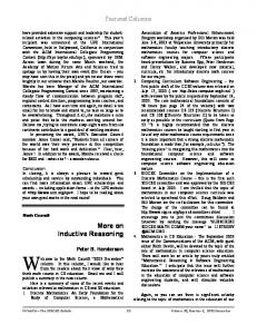
Both masks are of almost identical quality. This time, the mask shown in Matrix 31 was slightly ahead of the game, whereas the opposite was true when using the original training data subset. Figure 2 shows an almost perfect forecast throughout the testing period. In fact, the results are so good that the predicted data cannot be distinguished from the observed data
Peripheric resistance controller
International Journal of General Systems
847
Cardiovascular system 2
1.5
1
0
100
200
300
400
500
600
700
400
500
600
700
400
500
600
700
Time
Proximity
1
0.95
0.9
0
100
200
300 Time
Similarity
1 0.9 0.8 0.7
0
100
200
300 Time
Figure 2. PR controller of the cardiovascular system, first training data-set; (top) comparison of observed and predicted data, (centre) proximity measure of confidence in predictions made and (bottom) similarity measure of confidence in predictions made.
at all by the naked eye. The two confidence measures reflect this improvement as well. Although both confidence measures still have the largest doubts between samples 200 and 350, the confidence values now are never lower than 0.96, whereas before they had decreased to a value as low as 0.6 on one occasion.
3.2
Water demand time series
An FIR model has been obtained to predict the daily water demand of a section of the city of Barcelona (Lo´pez et al. 1996). The available measurement data contain the daily water demand of approximately 2 years. The demand is measured in m3. The city government was interested in making a prediction for 1 day ahead. Consequently, it made sense to perform an experiment in which the water demand for the following day is predicted by FIR, but then, the predicted value is immediately replaced by the true value, before yet another day is predicted. The experiment is described in detail in Lo´pez et al. (1996). No input variables are considered in the model. The water demand is treated as a time series. Future demand is predicted as a function of past demand only. 570 days (from 1 January 1985 to 24 July 1986) were used as training data, whereas 128 days (from 25 July 1986 to 29 November 1986) were used as testing data.
Barcelona water demand
848
F.E. Cellier et al.
2.5
Time series prediction
× 105
2 1.5 1
0
20
40
60
80
100
120
140
80
100
120
140
80
100
120
140
Time
Proximity
1 0.8 0.6 0.4
0
20
40
60 Time
Similarity
1 0.8 0.6 0.4 0.2 0
20
40
60 Time
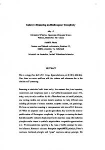
Figure 3. Water demand of the city of Barcelona; (top) comparison of observed and predicted data, (centre) proximity measure of confidence in predictions made and (bottom) similarity measure of confidence in predictions made.
The time series (solid line of Figure 3) shows a periodicity of 7 days. This makes sense, because, during the weekends, many companies are closed, and therefore, less water is being consumed. Also, the time series is mildly chaotic, i.e. no two weeks resemble each other totally. Figure 3 shows the forecast (dashed line) together with the measured values (solid line). Underneath, the two confidence measures are depicted. Contrary to the cardiology example, the relationship between the prediction error and the confidence measures is not immediately evident. Due to the chaotic nature of this time series, the confidence is generally lower than that in the cardiology example. The lower confidence values are primarily caused by a larger dispersion among the output values for similar inputs due to the chaotic nature of the data. In addition, the confidence is lower during weekends. This additional reduction in confidence is an artefact of data deprivation. There are only about 70 weekends among the training data, and thus, there are less near neighbours in the input space for weekend days than for week days. Hence, the additional reduction in confidence is caused by a lack of good neighbours in the input space, rather than by dispersion among the neighbours in the output space. Although the relationship between the prediction error and the two confidence measures is not evident to the naked eye, it can be shown statistically. To this end, the
International Journal of General Systems
849
cross-correlation between the prediction error and ð1:0 2 confi Þ was computed, where i stands for either proximity or similarity. How is the prediction error defined? There is not a unique formula that is commonly agreed upon to best represent a prediction error. Absolute errors and relative errors are widely used, but also mean square errors are commonly found. For the purpose of this investigation, a different error formula was used that balances well the different aspects of errors captured by the three aforementioned formulae and that also takes into account the dissimilarity between the curves representing the observed and the predicted trajectories. First, the observed testing data (meas) and the forecast testing data (pred) are jointly normalised to a range of [0.0, 1.0]: M ¼ maxðmeas; predÞ;
ð32Þ
m ¼ minðmeas; predÞ;
ð33Þ
mni ¼
measi 2 m ; M2m
ð34Þ
pni ¼
predi 2 m : M2m
ð35Þ
Then, the absolute error between the two normalised trajectories is computed: errabsi ¼ jmni 2 pni j:
ð36Þ
Due to the previous normalisation, the so computed absolute error can serve also as a measure of the relative error. Then, the dissimilarity error between the two normalised trajectories is computed: simtyi ¼
minðmni ; pni Þ ; maxðmni ; pni ; 1Þ
errsimi ¼ 1:0 2 simtyi :
ð37Þ ð38Þ
Finally, the overall error is computed as the mean of the two errors computed above: erri ¼
errabsi þ errsimi : 2
ð39Þ
The cross-correlation is computed using Matlab’s xcov function, as it is important to subtract the mean values of the two variables prior to computing their cross-correlation. The results are shown in Figure 4. It can be seen clearly that there exists a positive correlation between the two quantities at the centre, which is what was to be expected if the confidence measures are operating correctly. It can also be noticed that the correlation is a little higher in the case of the similarity measure, which is an indication of the somewhat higher sensitivity and reliability of this confidence measure. 4.
Discussion
The two examples presented above are useful in analysing the characteristics of the proposed confidence measures, as well as the capabilities of FIR for prediction in two very different situations. The CNS data correspond to a process that is largely deterministic, except at the peaks when the precise value is different from one period to the next, whereas
850
F.E. Cellier et al. Cross–correlation: prediction error (1–conf) 1
XCorr: proximity
0.8 0.6 0.4 0.2 0 –0.2 –0.4
0
50
100
150 dt
200
250
300
0
50
100
150 dt
200
250
300
XCorr: similarity
1.5 1 0.5 0 –0.5
Figure 4. Water demand of the city of Barcelona: cross-correlation between the prediction error and the confidence in the prediction made; (top) proximity measure and (bottom) similarity measure.
the water demand time series is mildly chaotic at all times. In a statistical sense, this time series can be interpreted as a stochastic quasi-stationary process. The value of confidence, using either of the two proposed confidence measures, is related to how deterministic the database is, i.e. how close or disperse the outputs are for any one input pattern. When the process to be modelled is mostly deterministic, FIR will have a high level of confidence in the predictions it makes. A reduction in confidence, in this situation, is a reflection of data deprivation, i.e. FIR does not find enough close neighbours in the experience database. More training data will solve the problem. On the other hand, if the system to be modelled is chaotic in nature, i.e. the measured data stream can be viewed as stochastic (though quasi-stationary), FIR will exhibit overall a lower confidence in its predictions. The reason for the reduced confidence here is the dispersion of outputs among the five nearest neighbours. Additional training data will not be able to solve this problem. 5. Conclusions When using FIR models in prediction, it is very important to generate not only forecasts for the output variables, but also measures of the reliability of each forecast. Two measures of confidence in the reliability of FIR predictions have been proposed in this paper, one being a proximity measure, the other being a similarity measure. After testing these measures on a largely deterministic SISO system and on a mostly stochastic time series, a few conclusions can be drawn:
International Journal of General Systems
851
. The similarity measure is more sensitive to the prediction error than the proximity measure. This is reasonable because the similarity measure preserves more information than the proximity measure about the qualitative difference between a new input state and its neighbours in the experience database. . Since the models derived by FIR are largely deterministic and autoregressive, in both the deterministic and the autoregressive stochastic processes, the proposed measures are useful tools to evaluate the likelihood of errors. More specifically, large proximity or similarity values indicate that a low prediction error is likely to occur. . In time series corresponding to stochastic processes that are not entirely autoregressive, i.e. processes where the errors may be correlated, there is not necessarily a significant correlation between the prediction error and ð1:0 2 confi Þ. Therefore, the correlation between these two entities may, in general, be used as an indicator of how well the series in question may be fitted by an autoregressive or deterministic model. A remark of a more philosophical nature is in place as well. The better the modelling methodology works, the less likely it is that a measure of the quality of the prediction can be made. If indeed the model were to exploit all the information that is available in the measurement data, then the model of the prediction error would necessarily have to behave like uncorrelated white noise, because whatever can be said about the prediction error can, at least in theory, be exploited to improve the model. In practice, this is not a big problem. As long as the prediction error does not behave like white noise, the information obtained is useful to assess the quality of the prediction. On the other hand, once the prediction error starts to behave like white noise, the modeller can be assured that he or she has exploited every bit of knowledge available, and has come up with the best possible model already. Hence even in that case, the error analysis reveals something of value. Acknowledgements The authors are thankful to Dr Rafael Huber of the Institute of Robotics and Industrial Informatics of the Polytechnical University of Catalonia for his continuous interest and support of this work. This project was in part sponsored by the Spanish Inter-ministerial Commission of Science and Technology (CICYT) through the project TAP96-0882: Seguridad de Funcionamiento en Sistemas Dina´micos Complejos.
Notes on contributors Franc¸ois E. Cellier received his BS degree in electrical engineering in 1972, his MS degree in automatic control in 1973, and his PhD degree in technical sciences in 1979, all from the Swiss Federal Institute of Technology (ETH) Zurich. Dr Cellier worked at the University of Arizona as professor of Electrical and Computer Engineering from 1984 until 2005. He then returned to his home country of Switzerland, where he is now once again working at his alma mater of ETH Zurich. Dr Cellier’s main scientific interests concern modelling and simulation methodologies, and the design of advanced software systems for simulation, computer-aided modelling and computer-aided design. Dr Cellier has authored or coauthored more than 250 technical publications, and he has edited several books. He published a textbook on Continuous System Modeling in 1991 and a second textbook on Continuous System Simulation in 2006, both with Springer-Verlag, New York.
852
F.E. Cellier et al. Josefina Lo´pez-Herrera obtained her PhD degree in advanced automation and robotics from the Polytechnical University of Catalonia, Barcelona, Spain in 1999. From 1988 until 2001, Dr Lo´pez worked as project leader in several Informatics Companies in Europe. She is currently assistant professor of software engineering at the Polytechnical University of Catalonia, Terrassa, Spain. Her research interests concern fuzzy systems, inductive reasoning and software design for advanced computational science.
` ngela Nebot received her BS and PhD degrees in computer science from A the Polytechnical University of Catalonia (UPC), Barcelona, Spain, in 1988 and 1994, respectively. She joined the Software Department of UPC in 1994 as an assistant professor, and since March 1998 she has been associate professor in the same department. She is currently the head of the soft-computing group. Her current research interests include fuzzy systems, neuro-fuzzy systems, genetic algorithms, simulation and e-learning. Dr Nebot served for several years on the editorial board of the journal ‘Simulation: Transactions of the Society for Modeling and Simulation International’ and she currently serves on the editorial board of the ‘International Journal of General Systems’. She collaborates as a reviewer with other international journals including ‘IEEE Transactions on Fuzzy Systems’, ‘Neurocomputing’, ‘Artificial Intelligence in Environmental Engineering’ and ‘Artificial Intelligence Communication’. Dr Nebot has authored or co-authored more than 80 technical publications. Gabriela Cembrano received her MS and PhD degrees from the Polytechnical University of Catalonia (UPC) in 1984 and 1988, respectively. Since 1989, she has been a tenured researcher of the Spanish National Research Council (CSIC) at the Institute of Robotics and Industrial Informatics. Her main research area is control engineering and she has been involved in industrial projects on modelling and optimal control of water supply, distribution and urban drainage systems since 1985. Currently, Dr Cembrano is also a member of CETAQUA – a water technology centre funded jointly by the water company Agbar, by UPC, and by CSIC – as head of one of four main research lines of the centre. She has taken part in several Spanish and European research projects in the field of advanced control and especially its application in water systems. She is now the main researcher of project ITACA (Integration of Advanced Techniques for Modelling, Supervision and Control in the Water Cycle) funded by the Spanish Ministry of Science and Education. She has published and co-authored various journal and conference papers in this field.
References Cellier, F.E., 1991. Continuous system modeling. New York: Springer-Verlag. Cellier, F.E. and Yandell, D.W., 1987. SAPS-II: a new implementation of the systems approach problem solver. International journal of general systems, 13, 307 –322. Cellier, F.E., et al., 1996a. Means for estimating the forecasting error in fuzzy inductive reasoning. Proceedings ESM’96, European simulation multiconference, 654–660. Ghent: SCS Europe BvbA.
International Journal of General Systems
853
Cellier, F.E., et al., 1996b. Combined qualitative/quantitative simulation models of continuous-time processes using fuzzy inductive reasoning techniques. International journal of general systems, 24, 95 – 116. Dubois, D. and Prade´, H., 1980. Fuzzy sets and systems, theory and applications. New York: Academic Press. Lo´pez, J., Cembrano, G. and Cellier, F.E., 1996. Time series prediction using fuzzy inductive reasoning. Proceedings ESM’96, European simulation multiconference. Ghent: SCS Europe BvbA, 765 – 770. MathWorks, I., 1993. Matlab: high-performance numeric computation and visualization software – user’s guide, Tech. rep., Natick, Mass. Nebot, A., Cellier, F.E. and Vallverdu´, M., 1998. Mixed quantitative/qualitative modeling and simulation of the cardiovascular system. Computer methods and programs in biomedicine, 55, 127 – 155.