Keywords: Fault tree analysis · Reliability modeling · Structure formulas ... For modern complex combinations of configurable hardware and software, modeling input is ..... basic event probabilities and the resulting configuration rankings?
Configurable Fault Trees oger, and Matthias Werner Christine Jakobs(B) , Peter Tr¨ Operating Systems Group, TU Chemnitz, Chemnitz, Germany {christine.jakobs,peter.troeger}@informatik.tu-chemnitz.de
Abstract. Fault tree analysis, as many other dependability evaluation techniques, relies on given knowledge about the system architecture and its configuration. This works sufficiently for a fixed system setup, but becomes difficult with resilient hardware and software that is supposed to be flexible in its runtime configuration. The resulting uncertainty about the system structure is typically handled by creating multiple dependability models for each of the potential setups. In this paper, we discuss a formal definition of the configurable fault tree concept. It allows to express configuration-dependent variation points, so that multiple classical fault trees are combined into one representation. Analysis tools and algorithms can include such configuration properties in their cost and probability evaluation. The applicability of the formalism is demonstrated with a complex real-world server system. Keywords: Fault tree analysis · Reliability modeling formulas · Configurable · Uncertainty
1
·
Structure
Introduction
Dependability modeling is an established tool in all engineering sciences. It helps to evaluate new and existing systems for their reliability, availability, maintainability, safety and integrity. Both research and industry have proven and established procedures for analyzing such models. Their creation demands a correct and detailed understanding of the (intended) system design. For modern complex combinations of configurable hardware and software, modeling input is available only late in the development cycle. In the special case of resilient systems, assumptions about the logical system structure may be even invalidated at run-time by reconfiguration activities. The problem can be described as uncertainty of information used in the modeling attempt. Such sub-optimal state of knowledge complicates early reliability analysis or renders it even impossible. Uncertainty is increasingly discussed in dependability research publications, especially in the safety analysis community. Different classes of uncertainty can be distinguished [16], but most authors focus on structural or parameter uncertainty, such as missing event dependencies [18] or probabilities. On special kind of structural uncertainty is the uncertain system configuration at run-time. From the known set of potential system configurations, it is unclear which one is used in practice. This problem statement is closely related c Springer International Publishing Switzerland 2016 � I. Crnkovic and E. Troubitsyna (Eds.): SERENE 2016, LNCS 9823, pp. 13–27, 2016. DOI: 10.1007/978-3-319-45892-2 2
14
C. Jakobs et al.
to classical phased mission systems [2] and feature variation problems known from software engineering. Configuration variations can be easily considered in classical dependability analysis by creating multiple models for the same system. In practice, however, the number of potential configurations seems to grow heavily with the increasing acceptance of modularized hardware and configurable software units. This demands increasing effort in the creation and comparison of all potential system variations. Alternatively, the investigation and certification of products can be restricted to very specific configurations only, which cuts down the amount of functionality being offered. We propose a third way to tackle this issue, by supporting configurations as explicit uncertainty in the model itself. This creates two advantages: – Instead of creating multiple dependability models per system configuration, there is one model that makes the configuration aspect explicit. This simply avoids redundancy in the modeling process. – Analytical approaches can vary the uncertain structural aspect to determine optimal configurations with respect to chosen criterias, such as redundancy costs, performance impact or resulting reliability. The idea itself is generic enough to be applied to different modeling techniques. In this paper, we focus on the extension of (static) fault tree modeling for considering configurations as uncertainty. This article relies on initial ideas presented by Tr¨ oger et al. [23]. In comparison, we present here a complete formal definition with some corrections that resulted from practical experience with the technique. We focus on the structural uncertainty aspect only and omit the fuzzy logic part from the original proposal here.
2
Clarifying Static Fault Trees
Fault trees are an ordered, deductive and graphical top-down method for dependability analysis. Starting from an undesired top event, the failure causes and their interdependencies are examined. A fault tree consists of logical symbols which either represent basic fault events, structural layering (intermediate events) or interdependencies between root causes (gates). Classical static fault trees only offer gates that work independent of the ordering of basic event occurence. Later extensions added the possibility for sequence-dependent error propagation logic [26]. Beside the commonly understood AND- and OR gates, there are some nonobvious cases in classical fault tree modeling. One is the XOR-gate that is typically only used with two input elements. Pelletrier and Hartline [19] proposed a more general interpretation we intend to re-use here:
Configurable Fault Trees
⎡ P (t) =
n � i=1
⎤⎤
⎡
⎢ ⎢ ⎢Pi (t) · ⎢ ⎣ ⎣
15
n �
j=1 j�=i
⎥⎥ ⎥ (1 − Pj (t))⎥ ⎦⎦
(1)
The formula for an XOR-gate sums up all variants where one input event is occurring and all the other ones are not. This fits to the linguistic definition of fault trees as model where “exactly one input event occurs” at a time [1]. The second interesting case is the Voting OR-gate, which expresses an error propagation when k-out-of-n input failure events occur. Equations for this gate type often assume equal input event probabilities [14], rely on recursion [17], rely on algorithmic solutions [4] or calculate only approximations [12,13] for the result. We use an adopted version of Heidtmanns work to calculate an exact result with arbitrary input event probabilities: P (k, n) =
n �
� � � i−1 · Pi (t) k−1
(−1)i−k ·
i=k
(2)
I∈Nj i∈I
As usual, if k = 1, the Voting OR-gate can be treated as an OR-gate. For k = n, the AND-gate formula can be used.
3
Configurable Fault Trees
Configurable fault trees target the problem of modeling architectural variation. It is assumed that the amount of possible system configurations is fixed and that it is only unknown which one is used. A configuration is thereby defined as set of decisions covering each possible architectural variation in the system. Opting for one possible configuration creates a system instance, and therefore also a dependability model instance. A system may operate in different instances over its complete life-time. 3.1
Variation Points
The configuration-dependent variation points are expressed by additional fault tree elements (see Table 1): A Basic Event Set (BES) is a model element summarizing a group of basic events with the same properties. The cardinality is expressed through natural numbers κ and may be explicitly given by the node itself, or implicitly given by a parent RVP element (see below). It can be a single number, list, or range of numbers. The parent node has to be a gate. The model element helps expressing an architectural variation point, typically when it comes to a choice of spatial redundancy levels. A basic event set node with a fixed κ is equivalent to κ basic event nodes.
16
C. Jakobs et al. Table 1. Additional symbols in configurable fault trees.
Basic Event Set (BES): Set of basic events with identical properties. Cardinality is shown with a # symbol. Intermediate Event Set (IES): Set of intermediate events having identical subtrees. Cardinality is shown with a # symbol. Feature Variation Point (FVP): 1-out-of-N choice of a subtree, depending on the configuration of the system. Redundancy Variation Point (RVP): Extended Voting OR-gate with a configuration-dependent number of redundant units. Inclusion Variation Point (IVP): Event or event set that is only part of the model in some configurations, expressed through dashed lines.
An Intermediate Event Set (IES) is a model element summarizing a group of intermediate events with the same subtree. When creating instances of the configurable fault tree, the subtree of the intermediate event set is copied, meaning that the replicas of basic events stand for themselves. A typical example would be a complex subsystem being added multiple times, such as a failover cluster node, that has a failure model on its own. An intermediate event set node with a fixed κ is equivalent to κ transfer-in nodes. A Feature Variation Point (FVP) is an expression of architectural variations as choice of a subtree. Each child represents a potential choice in the system configuration, meaning that out of the system parts exactly one is used. An interesting aspect are event sets as FVP child. Given the folding semantic, one could argue that this violates the intended 1-out-of-N configuration choice of the gate, since an instance may have multiple basic events being added as one child [23]. This argument doesn’t hold when considering the resolution time of parent links. The creation of an instance can be seen as recursive replacement activity, were a chosen FVP child becomes the child of a higher-level classical fault tree gate. Since the BES itself is the child node, the whole set of ‘unfolded’ basic events become child nodes of the classical gate. Given that argument, it is valid to allow event sets as FVP child. A Redundancy Variation Point (RVP) is a model element stating an unknown level of spatial redundancy. As extended Voting OR-gate, it has the number of elements as variable N and a formula that describes the derivation of k from a given N (e.g. k = N − 2). All child nodes have to be event sets with unspecified cardinality, since this value is inherited from the configuration choice in the parent RVP element. N can be a single number, list or range of numbers. A RVP with a fixed N is equivalent to a Voting OR-gate. If a transfer-in element is used as child node, the included fault tree is inserted as intermediate event set.
Configurable Fault Trees
17
An Inclusion Variation Point (IVP) is an event or event set that, depending on the configuration, may or may not be part of the model. In contrast to house events, the failure probability is known and only the occurrence in the instance is in doubt. An IVP is slightly different to the usage of an FVP, since the former allows configurations where none of the childs is a part of the failure model. In this case, the parent gate is (probably recursively) vanished from the model instance. Classical Voting OR-gates with an IVP child can no longer state an explicit N , since this is defined from the particular configuration. This is the only modification of classical fault tree semantics reasoned by our extension. 3.2
Mathematical Representation
A configuration can be understood as a set of mappings from a variation point node to some specific choice. Depending on the node type, an inclusion variation point can be enabled or disabled, one child has to be selected at a feature variation point, or N and therefore also k is specified for a redundancy variation point. Event sets, whether BES or IES, are a folded group that translate to single events in one instance. Since there is no difference between an event and an event set with cardinality of one, it is enough to discuss the formal representation of the latter only. The cardinality of event sets is represented through # in the model, while in the mathematical description κ is used. The formal representation of classical AND and OR gates needs to include the cardinality κ of a potential BES or IES child: P (t) =
n �
Pi (t)κi ; κi ∈ N
(3)
i=1
P (t) = 1 −
n �
[1 − Pi (t)]κi ; κi ∈ N
(4)
i=1
For classical XOR gates, we rely on Eq. 1 as starting point. In addition, the κ value of child nodes also has to be considered: P (t) =
n �� n � (1 − Pl (t))κl κi · Pi (t) · l=1 ; (1 − Pi (t)) i=1
(5)
f or κi , κl ∈ N; Pi (t) �= 1 The summation term goes over each gate (i = 1 to n) and declares a summation part for the output = true case in the truth table for this gate. As the child can be a BES with a cardinality greater than one, there would be one summation part for each cardinality, which can be rewritten as κi times the output = true line in the truth table. Also the product part of the formula needs to be exponentiated. All other combinations are eliminated from the calculation. To make the equation valid for general use in algorithms, the event probability processed at the very moment has to be divided once from the product
18
C. Jakobs et al.
part of the formula. This makes it unnecessary to clarify which event given what cardinality is processed at the moment. Such an approach is only valid as long as the component probability is smaller than one, which seems to be a reasonable assumption in dependability modeling. The Voting OR-gate has to be analyzed by calculating all possible failure combinations. With Eq. 2 in mind, a reduced calculation is possible. When using BES nodes as child, the different instances according to the cardinality have to be considered. This is done by defining first a set of sub-sets Nx which represents the combinations of the event indexes and the cardinality indexes. Given that, we redefine the specification of Nj to be the set of all combinations of sub-sets of Nx : P (k, n) =
m � i=k
� � � i−1 · · Pi (t) k−1
i−k
(−1)
(6)
I∈Nj i∈I
For special cases k = 1 or k = N , the according equations for OR and AND gates can be used respectively. The FVP represents a variable point in the calculation that is defined by one sub-equation and the κ value for a given instance. This allows to represent the FVP with a single indexed variable. The RVP expresses uncertainty about the needed level of redundancy. It is an extended form of the Voting OR-gate. The structural uncertainty is represented by the possibilities for the N value that influence the k-formula. A new variable is therefore defined which gets the different results as a value, so that the impact of the redundancy variation is kept till the end of the analysis. An RVP with a single value for N is a Voting OR-gate. The IVP states an uncertainty about whether the events or underlying subtrees will be part of the system or not. It is formally represented by a variable that can either stand for the event probability or the neutral probability in case the IVP acts as non-included.
4
Use Case Example
The use case example is a typical high-performance server system available in multiple configurations1 . The main tree is shown in Fig. 1. Two subtrees are included by the means of standard transfer-in gates. We only show a qualitative fault tree here, but the formula representations can be used to derive quantitative results, too. It should be noted that intermediate events only serve as high-level description of some event combination, although they map to higher-order configurations in the example case. The server has a hot swap power supply, so the machine fails if both power supplies are failing at the same time. The cardinality is defined by the BES node itself, so: 1
https://www.thomas-krenn.com/en/wiki/2U Intel Dual-CPU RI2212+ Server.
Configurable Fault Trees
19
Server Failure
Hot Swap Power Supply (hotswap)
Supermicro X10DRCLN4+ Mainboard (mainboard)
RAM Failure
RAID Failure
1-Port LAN (τlan1 )
2-Port LAN (τlan2 )
4-Port LAN (τlan4 )
CPU Configuration (τcpu )
920 W (pwr) #2
E5-2623v3 E5-2603v3 E5-2609v3 E5-2620v3 E5-2643v3 4-Core 6-Core 6-Core 6-Core 6-Core 3,0 GHz 1,6 GHz 1,9 GHz 2,4 GHz 3,4 GHz (cpu2623 ) (cpu2603 ) (cpu2609 ) (cpu2620 ) (cpu2643 ) #2 #2 #2 #2 #2
E52630Lv3 8-Core 1,8 GHz (cpu2630L ) #2
E5-2630v3 E5-2640v3 E5-2650v3 E5-2670v3 E5-2690v3 E5-2695v3 8-Core 8-Core 10-Core 12-Core 12-Core 14-Core 2,4 GHz 2,6 GHz 2,3 GHz 2,3 GHz 2,6 GHz 2,3 GHz (cpu2630 ) (cpu2640 ) (cpu2650 ) (cpu2670 ) (cpu2690 ) (cpu2695 ) #2 #2 #2 #2 #2 #2
Fig. 1. Main tree for RI2212+ server
hotswap = pwr2
(7)
For the CPU variation point, a variable is defined based on the current configuration choice, expressed by the function ch(): ⎧ ⎪ cpu2623 , κcpu = 2; if ch(τcpu ) = 1 ⎪ ⎨ τcpu = cpu2603 , κcpu = 2; if ch(τcpu ) = 2 (8) ⎪ ⎪ ⎩... The server can be optionally equipped with additional LAN cards, which is described in a similar way.
20
C. Jakobs et al.
RAM Failure
RAM Configuration (τram )
4 GB Modules (ms4gb)
8 GB Modules (ms8gb)
16 GB Modules (ms16gb)
Standard / Premium
4GB ECC DDR4 (m4gb) #2,4
32 GB Modules (ms32gb)
Standard / Premium
16GB ECC DDR4 (m16gb) #2,4,8,16 8GB ECC DDR4 (m8gb) #2,24
8GB ECC DDR4 Premium (m8gbp) #2
32GB ECC DDR4 Premium (m32gbp) #2,4,8,16,24
32 GB ECC DDR4 (m32gb) #24
Fig. 2. Subtree for server RAM configurations
As for the CPU, the RAM can be configured in many different ways (see Fig. 2). The failure events for single modules are expressed as event sets with a direct list of cardinalities. This is reflected in the related equation system:
τm4gb
� m4gb, κm4gb = 2; if ch(τm4gb ) = 1 = m4gb, κm4gb = 4; if ch(τm4gb ) = 1
ms4gb = 1 − (1 − m4gb)κm4gb � m8gb, κm8gb = 2; if ch(τm8gb ) = 1 τm8GB = m8gb, κm8gb = 24; if ch(τm8gb ) = 1 ⎧ κm8gb ⎪ ; ⎨1 − (1 − m8gb) τms8gb = if ch(τms8gb ) = 1 ⎪ ⎩ 1 − (1 − m8gbp)2 ; if ch(τms8gb ) = 2 ms8gb = τms8gb ...
(9) (10) (11)
(12) (13)
Configurable Fault Trees
τRAM
⎧ ⎪ ⎪ms4gb; if ch(τRAM ) = 1 ⎪ ⎨ms8gb; if ch(τ RAM ) = 2 = ⎪ms16gb; if ch(τRAM ) = 3 ⎪ ⎪ ⎩ ms32gb; if ch(τRAM ) = 4
21
(14)
The RAID subtree (see Fig. 3) in combination with the hard disc subtree (ommitted due to space restrictions) expresses configuration modes of the RAID controller, were each of them relies on some predefined variation for the number of discs. The determination of τdisc works similarly to the approach shown with τcpu (see Eq. 8). The more interesting aspect is the representation of the different RAID configurations.
RAID Failure
RAID Controller
RAID Configuration (τRAID )
Cache Vault Module (τcache )
raid0
raid1
raid5
raid6
raid10
raid50
raid60
Nraid0 : 2 − 12 k : 1
Nraid1 : 2 − 12 k : N
Nraid5 : 3 − 12 k : 2
Nraid6 : 4 − 12 k : 3
Nraid10 : 2−6 k : 1
Nraid50 : 2−4 k : N −1
Nraid60 : 1−2 k : N −1
Discs
Discs
Discs
Discs
subraid1
subraid5
subraid6
N: 2, k: 2
N: 3, k: 2
N: 4, k: 3
Discs
Discs
Discs
Fig. 3. Sub tree for server RAID configurations.
22
C. Jakobs et al.
RAID 0 and RAID 1 are special cases. In the RAID 0 case, the variation point can be interpreted as OR-gate. For RAID 1, the variation point can be interpreted as AND-gate: ⎧ [1 − (1 − τdisc )2 ]; if ch(Nraid0 ) = 2 ⎪ ⎪ ⎪ ⎪ ⎨[1 − (1 − τdisc )3 ]; if ch(Nraid0 ) = 3 raid0 = . (15) ⎪.. ⎪ ⎪ ⎪ ⎩ [1 − (1 − τdisc )12 ]; if ch(Nraid0 ) = 12 ⎧ 2 ⎪ ⎪(τdisc ) ; if ch(Nraid1 ) = 2 ⎪ ⎪ ⎨(τdisc )3 ; if ch(Nraid1 ) = 3 (16) raid1 = . .. ⎪ ⎪ ⎪ ⎪ ⎩ (τdisc )12 ; if ch(Nraid1 ) = 12 RAID 5 and RAID 6 are based on striping and parity bits and fail if two respectively three disks fail. Since both RAID types lead to the same mathematical representation, we show only one here: ⎧ ⎪ = τdisc1,1 τdisc1,2 + τdisc1,1 τdisc1,3 + ⎪ ⎪ ⎪ ⎪ ⎪ ⎪τdisc1,2 τdisc1,3 − 2 · (τdisc1,1 τdisc1,2 ⎪ ⎪ ⎪ ⎪τdisc1,3 ); if ch(Nraid5 ) = 3 ⎪ ⎪ ⎪ ⎪ ⎪ ⎪ ⎪ ⎪ ⎪ = τdisc1,1 τdisc1,2 + ⎪ ⎪ ⎪ ⎪ ⎪ τ + τdisc1,1 τdisc1,4 + τ ⎪ ⎨ disc1,1 disc1,3 raid5 = τdisc1,2 τdisc1,3 + τdisc1,2 τdisc1,4 + ⎪ ⎪ ⎪τdisc1,3 τdisc1,4 − 2 · (τdisc1,1 τdisc1,2 ⎪ ⎪ ⎪ ⎪τdisc1,3 + τdisc1,1 τdisc1,2 τdisc1,4 + ⎪ ⎪ ⎪ ⎪ ⎪ τdisc1,1 τdisc1,3 τdisc1,4 + τdisc1,2 ⎪ ⎪ ⎪ ⎪ ⎪ τ disc1,3 τdisc1,4 ) + 3(τdisc1,1 τdisc1,2 ⎪ ⎪ ⎪ ⎪ ⎪ τdisc1,3 τdisc1,4 ); if ch(Nraid5 ) = 4 ⎪ ⎪ ⎪ ⎪ ⎩...
(17)
RAID 10, 50 and 60 are based on two levels. The lower one is an RAID 1, 5 or 6 and the upper one is RAID 0. We show the RAID 10 case as example, the others are comparable:
Configurable Fault Trees
2 subraid1 = τdisc ⎧ [1 − (1 − subraid1)2 ]; ⎪ ⎪ ⎪ ⎪ ⎪ if ch(Nraid10 ) = 2 ⎪ ⎨ [1 − (1 − subraid1)3 ]; raid10 = ⎪ ⎪ if ch(Nraid10 ) = 3 ⎪ ⎪ ⎪ ⎪ ⎩.. .
23
(18)
(19)
The FVP node expresses the single choice for one of the RAID configurations: ⎧ raid0; if ch(modraid) = 1 ⎪ ⎪ ⎪ ⎪ ⎨raid1; if ch(modraid) = 2 (20) τmodraid = . .. ⎪ ⎪ ⎪ ⎪ ⎩ raid60; if ch(modraid) = 7 The Cache Vault Module can be added to the server to get a battery-backed write cache in the RAID controller. It is represented as IVP. Similar to the voter in a triple modular redundancy setup, it can act both as source of reliability and additional root cause for a system failure. Since the parent node is an OR-gate, the value may become 0, since this is the neutral element for OR-parents: � cache; if ch(cache) = 1 (true) τcache = (21) 0; if ch(cache) = 0 (false) The complete RAID system then ends up being expressible like this: τRAID = 1 − [(1 − RAIDController )· (1 − τmodraid ) · (1 − τcache )]
(22)
At last, the server itself can be evaluated through the OR-gate equation. Combining all sub parts, the overall server structure formula representing the configurable fault tree looks like this: Server F ailure = 1 − [(1 − hotswap) · (1 − mainboard)· (1 − τcpu ) · (1 − τRAM ) · (1 − τlan1 )· (1 − τlan2 ) · (1 − τlan4 ) · (1 − τRAID )]
(23)
The stated set of expressions represents 4.259.520 possible server configurations, which would otherwise needed to be modeled in single fault trees. Based on the given expression, it would now be interesting to determine configurationdependent and independent cut sets. Furthermore, each configuration may be related to some costs, f.e. based on the components being involved. The following section discussed some options for such analysis tasks.
24
5
C. Jakobs et al.
Analyzing Configurable Fault Trees
Configurable fault trees can obviously be analyzed by enumerating all possible configurations, creating the structure formula for each of them and treating the resulting set as equation system [23]. By iterating over the complete configuration space, best and worst cases can be identified in terms of their variation point settings. Especially if configuration parameters depend on each other, this kind of analysis can be helpful to deduct system design decisions. Similarly, it is possible to do an exhaustive analysis of cut sets for each of the configurations. This allows to identify configuration-dependent and configuration-independent cuts sets for the given fault tree model as a whole. An easy addition to the presented concept is a cost function. It may express component or manufacturing costs, energy needed for operating the additional component, repair costs if the component fails, or — in case of the top event — the cost introduced by the occurrence of a failure. The opposite approach is also possible. Each failure model element can be extended with a performance factor, which should be maximized for the whole system. Adding some system part in a configuration may then decrease the failure probability and decrease the performance at the same time. This again allows automated trade-off investigations for the system represented by the configurable fault tree. A typical analysis outcome in classical fault trees are importance metrics. They determine basic events that have the largest impact to the failure probability of the system [8,20]. Classical importance metrics assume a coherent fault tree that is translated to a linear structure formula. In case of configurable fault trees, there are two factors that may have impact: Basic events and configuration changes. One algebraic way for such analysis is the Birnbaum reliability importance measure in its rewritten version for pivotal decomposition [5]. It can determine the importance of a configurable element in the structure formula. The creation of a combined importance metric for basic events and configuration changes raises some challenges. The reason for the non-applicability of classical importance measures here is the discontinuity in an importance function in combination with possibly existing trade-offs between configuration and basic probabilities. The impact of selecting a specific configurations may depend on the probability of basic events. A simple example is a feature variation point that either enables or disables the usage of a Triple Modular Redundancy (TMR) structure. Depending on the failure probability of the voter and the replicated modules, the configuration with TMR might decrease or increase the system failure probability. This leads to an interesting set of new questions: – Is there a dominating configuration that always provides the best (worst) result for the overall space of basic event probabilities? – If so, how can it be identified without enumerating the complete space of configurations? – If not, what are the numerical dependencies between configuration choices, basic event probabilities and the resulting configuration rankings?
Configurable Fault Trees
25
– Given that, how is the importance of a particular event related to configuration choices? The answer to these questions as well as a general importance metric is part of our future work on the topic.
6
Related Work
Ruijters and Stoelinga [21] created an impressive summary of fault tree modeling approaches and their extensions, covering things such as the expression of timing constraints or unknown basic probabilities. Although many different kinds of uncertainty seemed to be discussed for fault trees, we found no consideration of parametric uncertainty. Bobbio et al. [6] addressed the problem of fault trees for big modern systems. They propose the folding of redundant fault tree parts, but their approach cannot handle true architecture variations. Buchacker [10] uses finite automata at the leaves of the fault tree to model interactions of basic events. The automata can be chosen from a predefined set or custom sub-models. This makes it possible to model basic events affecting each other, but only in one configuration. Kaiser et al. [15] introduced the concept of components in fault trees, by modeling each of them in a separate tree. This supports a modular and scalable system analysis, but does not target the problem of parametric uncertainties. An interesting attempt for systems with dynamic behavior is given by Walter et al. [25]. The proposed textual notation for varying parts may serve as suitable counterpart for the graphical notation proposed here. In [9], continuous gates are used to model relationships between elements of a fault tree. This is divergent to our uncertainty focus, but the approach might be useful as an extension in future work. There are several existing approaches for considering uncertainty in importance measures, which “reflect to what degree uncertainty about risk and reliability parameters at the component level influences uncertainty about parameters at the system level” [11]. Walley [24] gives an overview over different uncertainty measures which can be used in expert systems. The presented metrics are based on Bayesian probabilities, coherent lower previsions, belief functions and possibility measures. Borgonovo [7] examined different uncertainty importance measures based on InputOutput correlation or Output variance. Suresh et al. [22] proposed to modify importance measures for the use with fuzzy numbers. Baraldi et al. [3] proposed a component ranking by Birnbaum importance in systems with uncertainty in the failure event probabilities. All these approaches do examine the value of the output uncertainty which respect to the uncertain input values, which relates to parameter, but not parametric uncertainty as in our case.
7
Conclusion and Future Work
We presented an approach for expressing different system configurations directly as part of a fault tree model. The resulting configurable fault tree allows the
26
C. Jakobs et al.
derivation of failure model instances, where each of them describes the dependability of a particular system configuration. Based on clarified semantics for XOR and Voting OR-gates, we have shown how configurable fault trees can be represented both graphically and mathematically. We offer a web-based tool2 for evaluating the modeling concept. The underlying open source project3 is available for public use and further development. The most relevant next step is the formal definition of analytical metrics that comply with the configuration idea. Unfortunately, dependencies in the configuration space can not yet be expressed explicitly. This flaw already appeared in the presented use case, where certain CPU models are only usable with certain RAM constellations. We can imagine to express such dependencies by abusing house events as ‘switches’, but it doesn’t seem to be appropriate. Instead, we intend to extend the modeling approach in the future for supporting an explicit expression of the relations, either at modeling or analysis time.
References 1. DIN EN 61025:2007 Fehlzustandsbaumanalyse (2007) 2. Band, R.A.L., Andrews, J.D.: Phased mission modelling using fault tree analysis. In: Proceedings of the Institution of Mechanical Engineers (2004) 3. Baraldi, P., Compare, M., Zio, E.: Component ranking by Birnbaum importance in presence of epistemic uncertainty in failure event probabilities. IEEE Trans. Reliab. 62, 37–48 (2013) 4. Barlow, R.E., Heidtmann, K.D.: Computing k-out-of-n reliability. IEEE Trans. Reliab. R–33(4), 322 (1984) 5. Birnbaum, Z.: On the importance of different components in a multicomponent system. Laboratory of Statistical Research, Department of Mathematics, University of Washington, Seattle, Washington (1968). No. 54 6. Bobbio, A., Codetta-Raiteri, D., Pierro, M.D., Franceschinis, G.: Efficient analysis algorithms for parametric fault trees. In: 2005 Workshop on Techniques, Methodologies and Tools for Performance Evaluation of Complex Systems (FIRB-PERF 2005), pp. 91–105 (2005) 7. Borgonovo, E.: Measuring uncertainty importance: investigation and comparison of alternative approaches. Risk Anal. 26(5), 1349–1361 (2006) 8. van der Borst, M., Schoonakker, H.: An overview of PSA importance measures. Reliab. Eng. Syst. Safety 72(3), 241–245 (2001) 9. Brissaud, F., Barros, A., B´erenguer, C.: Handling parameter and model uncertainties by continuous gates in fault tree analyses. Proc. Inst. Mech. Eng. Part O J. Risk Reliab. 224(4), 253–265 (2010) 10. Buchacker, K.: Modeling with extended fault trees. In: Fifth IEEE International Symposium on High Assurance Systems Engineering (HASE 2000), pp. 238–246 (2000) 11. Flage, R., Terje, A., Baraldi, P., Zio, E.: On imprecision in relation to uncertainty importance measures. In: ESREL, pp. 2250–2255 (2011) 2 3
https://www.fuzzed.org. https://github.com/troeger/fuzzed.
Configurable Fault Trees
27
12. Heidtmann, K.D.: A class of noncoherent systems and their reliability analysis. In: 11th Annual Symposium on Fault Tolerant Computing, pp. 96–98 (1981) 13. Heidtmann, K.D.: Improved method of inclusion-exclusion applied to k-out-of-n systems. IEEE Trans. Reliab. R–31(1), 36–40 (1982) 14. Hoang, P., Pham, M.: Optimal designs of {k, n−k+1}-out-of-n: F systems (subject to 2 failure modes). IEEE Trans. Reliab. 40(5), 559–562 (1991) 15. Kaiser, B., Liggesmeyer, P., M¨ ackel, O.: A new component concept for fault trees. In: Proceedings of the 8th Australian Workshop on Safety Critical Systems and Software (SCS 2003), vol. 33, pp. 37–46 (2003) 16. Kennedy, M.C., O’Hagan, A.: Bayesian calibration of computer models. J. R. Stat. Soc. Ser. B (Statistical Methodology) 63(3), 425–464 (2001) 17. Malinowski, J.: A recursive algorithm evaluating the exact reliability of a circular consecutive k-within-m-out-of-n: F system. Microelectron. Reliab. 36(10), 1389– 1394 (1996) 18. Pedroni, N., Zio, E.: Uncertainty analysis in fault tree models with dependent basic events. Risk Anal. 33(6), 1146–1173 (2013) 19. Pelletier, F.J., Hartline, A.: Ternary exclusive OR. Logic J. IGPL 16(1), 75–83 (2008) 20. Rausand, M., Høyland, A.: System Reliability Theory: Models, Statistical Methods and Applications. Wiley-Interscience, Hoboken (2004) 21. Ruijters, E., Stoelinga, M.: Fault tree analysis: a survey of the state-of-the-art in modeling, analysis and tools. Proc. Inst. Mech. Eng. Part O J. Risk Reliab. 224(4), 253–265 (2010) 22. Suresh, P.V., Babar, A.K., Raj, V.V.: Uncertainty in fault tree analysis: a fuzzy approach. Fuzzy Sets Syst. 83, 135–141 (1996) 23. Tr¨ oger, P., Becker, F., Salfner, F.: Fuzztrees - failure analysis with uncertainties. In: 2013 IEEE 19th Pacific Rim International Symposium on Dependable Computing, pp. 263–272 (2013) 24. Walley, P.: Measures of uncertainty in expert systems. Artif. Intell. 83(1), 1–58 (1996) 25. Walter, M., Gouberman, A., Riedl, M., Schuster, J., Siegle, M.: Lares — a novel approach for describing system reconfigurability in dependability models of faulttolerant systems. In: Proceedings of European Safety and Reliability Conference (ESREL 2009) (2009) 26. Xiang, F., Machida, F., Tadano, K., Yanoo, K., Sun, W., Maeno, Y.: A static analysis of dynamic fault trees with priority-and gates. In: 2013 Sixth Latin-American Symposium on in Dependable Computing (LADC), pp. 58–67 (2013)
http://www.springer.com/978-3-319-45891-5