Conflict Resolution a First-Order Resolution Calculus with Decision Literals and Conflict-Driven Clause Learning John Slaney
Bruno Woltzenlogel Paleo
arXiv:1602.04568v1 [cs.LO] 15 Feb 2016
Australian National University
[email protected] [email protected]
Abstract This paper defines the (first-order) conflict resolution calculus: an extension of the resolution calculus inspired by techniques used in modern SAT-solvers. The resolution inference is restricted to (first-order) unit-propagation and the calculus is extended with a mechanism for assuming decision literals and a new inference rule for clause learning, which is a first-order generalization of the propositional conflict-driven clause learning (CDCL) procedure. The calculus is sound (because it can be simulated by natural deduction) and refutationally complete (because it can simulate resolution), and these facts are proven in detail here. Categories and Subject Descriptors F.4.1, I.2.3 [mathematical logic, deduction and theorem proving]: proof theory, deduction Keywords Proof Theory, Resolution, Natural Deduction, SAT, First-Order Logic, Conflict-Driven Clause Learning
1.
Introduction
Modern SAT-solvers are famously efficient for solving the decision problem of satisfiability of propositional formulas, and we may wonder whether the ideas used in SAT-solvers could be generalized to the first-order case. This paper addresses this question from a purely proof-theoretical perspective. We briefly recall the first-order resolution calculus (in Section 2), which is the theoretical foundation for many current state-ofthe-art first-order theorem provers (e.g. (Riazanov and Voronkov 2002; Schultz 2013; Weidenbach et al. 2009)), and the DPLL and CDCL procedures used by SAT-solvers (in Section 3). The main contribution of this paper (presented in Section 4) is the conflict resolution calculus CR. It extends the first-order resolution calculus with decision literals and a new inference rule for clause learning and restricts the resolution rule in order to force it to behave like unit propagation. As discussed in Subsection 4.1, a certain subclass of CR derivations is isomorphic to the abstract data structure known as conflict graphs or implication graphs and widely used to describe the procedures of modern SAT-solvers. Furthermore, as shown in Section 7, whereas the splitting technique used by modern first-order provers must either be handled at an extra-logical level
Permission to make digital or hard copies of part or all of this work for personal or classroom use is granted without fee provided that copies are not made or distributed for profit or commercial advantage and that copies bear this notice and the full citation on the first page. Copyrights for components of this work owned by others than ACM must be honored. Abstracting with credit is permitted. To copy otherwise, to republish, to post on servers, or to redistribute to lists, contact the Owner/Author. Request permissions from
[email protected] or Publications Dept., ACM, Inc., fax +1 (212) 869-0481. Copyright 20yy held by Owner/Author. Publication Rights Licensed to ACM. CONF ’yy Month d–d, 20yy, City, ST, Country c 20yy ACM 978-1-nnnn-nnnn-n/yy/mm. . . $15.00 Copyright DOI: http://dx.doi.org/10.1145/nnnnnnn.nnnnnnn
or lead to an unacceptable increase in proof size if simulated in the resolution calculus, its simulation by CR’s decisions and clause learning is lean and straightforward. Therefore, the new CR calculus provides a more adequate proof-theoretical foundation for procedures currently implemented by SAT-solvers and first-order provers. In CR, it becomes evident that decision literals are analogous to assumptions in natural deduction, whereas clause learning resembles natural deduction’s implication introduction rule. This fact is crucial for the proof of soundness of CR (shown in Section 6) and it illustrates an insightful novelty of the calculus: while the resolution inference proposed by Robinson (1960) can be regarded as a first-order generalization of modus ponens (a.k.a. natural deduction’s implication elimination) by taking unification into account, the clause learning rule proposed here (and inspired by the propositional CDCL technique) can be considered a first-order generalization of implication introduction, as it discharges decision literals in a way that allows for unification. Any resolution refutation can be translated into a refutation in the proposed calculus. Therefore, CR’s refutational completeness follows easily from the refutational completeness of the resolution calculus (as demonstrated in Section 5). A main motivation for the development of the conflict resolution calculus was that it might eventually serve as a theoretical common ground for existing first-order provers that try to harness or mimic the power of SAT-solvers (cf. Section 9)) or as a starting point for the development of new provers, in the same way that the pure resolution calculus provided the basic foundation for several generations of automated theorem provers in the last decades. To achieve this goal, the calculus is presented in a general way, avoiding premature optimizations and refinements, so that future work may easily build on it and explore various proof search strategies and implementation techniques.
2.
Recalling Resolution
Clauses (denoted c, possibly subscripted) are disjunctions of literals. A literal is either an atom or a negated atom, and an atom is a n-ary predicate (denoted P or Q) applied to n terms. A term is either a constant (denoted a or b), a variable (denoted x, y, v or z) or an n-ary function (denoted f or g) applied to n terms. Variables in a clause are assumed to be implicitly universally quantified. A clause having a single literal is called unit. If ` is a literal, ` denotes its dual (i.e. P = ¬P and ¬P = P ). The nullary atoms > (verum) and ⊥ (falsum) have special meanings characterized by the following equations: Γ ∨ ⊥ = Γ and Γ ∨ > = >. All inference rules operating on clauses are assumed to be modulo disjunction’s associativity and commutativity, modulo negation’s involutivity and modulo the equations for > and ⊥. The empty clause is logically equivalent
to the clause containing only ⊥. Therefore, slightly abusing notation, it is denoted by ⊥. Substitutions (denoted by σ, possibly suband superscripted) are assumed to implicitly avoid variable capture. The empty (i.e. identity) substitution is denoted ε. The inference rules of the resolution calculus are shown in Fig. 1. A resolution proof of a clause c from a set of clauses S is a directed acyclic graph (DAG) where leaves (i.e. input nodes) are clauses from S, internal nodes are obtained from their parents through application of the inference rules and the sink node is the clause c. A resolution refutation of a set of clauses S is a proof of the empty clause (denoted ⊥) from S. It is assumed that distinct input clauses do not share variables. Furthermore, the inference rules implicitly generate fresh symbols for variables, thereby maintaining the invariant that distinct clauses do not share variables. Proof DAGs are sometimes displayed as a collection of trees according to the following convention: nodes used as premises more than once are given names (e.g. ϕ, ψ or ξ) when they are used for the first time, and the names are used to refer to the nodes whenever they are used again. By naming and referring, wide proof trees can also be broken down in smaller displayable parts. Example 1. Consider a proof with the following non-tree form:
It can be displayed as the single tree with names and references below, where the second (rightmost) occurrence of the name ψ is to be understood as a reference to the node named ψ by the first (leftmost) occurrence of ψ: c1
c2 ψ : c4
c3
ψ
c6
c5 c7
c8 Or it can also be displayed as the following forest, where the two occurrences of the name ψ in the lower tree are to be understood as references to the node named ψ in the upper tree: c1
c2 ψ : c4
c3 c6
where σ is a unifier of ` and `0 . Factoring: `1 ∨ . . . ∨ `n ∨ `01 ∨ . . . ∨ `0m f (σ) (` ∨ `01 ∨ . . . ∨ `0m ) σ where σ is a unifier of `1 , . . . `n and ` = `k σ, for any k ∈ {1, . . . , n}. Figure 1. Resolution Calculus efforts culminated in the superposition1 calculus (Bachmair and Ganzinger 1990, 1994; Waldmann 2015), which extends the resolution calculus with a paramodulation rule (Robinson and Wos 1969) for equality reasoning and refines it with ordering restrictions on terms and literals. Another practical problem is that the resolvent of a clause with n literals and another clause with m literals has n + m − 2 literals. When iterated, this results in very long clauses and, consequently, a loss of efficiency. This practical problem has been solved with a technique known as splitting (Weidenbach 2001): if the current set of clauses is S ∪ {Γ1 ∨ . . . ∨ Γk } and the sets of variables Vi of Γi are mutually disjoint, then we can split the long clause Γ1 ∨ . . . ∨ Γk into its variable-disjoint components and the clause set into the k sets S ∪ {Γi } (for 1 ≤ i ≤ k). The disjointness of the sets of variables Vi ensures that we can check the unsatisfiability of each resulting clause set independently: S ∪ {Γ1 ∨ . . . ∨ Γk } is unsatisfiable iff S ∪ {Γi } is unsatisfiable for every variable-disjoint component Γi . From a proof-theoretical perspective, splitting resembles the β-rule of free-variable tableaux (Beth 1955; Weidenbach 2002). Therefore, superposition provers that implement splitting (Weidenbach et al. 2009; Schultz 2013; Riazanov and Voronkov 2002) can be seen as hybrids combining resolution/superposition and tableaux. Up to now, however, there has been no single pure proof system capable of characterizing what is going on inside a modern state-of-the-art first-order theorem prover. This gap between theory and practice is something that can be remedied with the adoption of the CR calculus proposed here (cf. Section 7).
3. ψ
ψ
Resolution: Γ ∨ ` `0 ∨ ∆ r(σ) (Γ ∨ ∆) σ
c5 c7
c8 Given a set of clauses, a resolution prover exhaustively applies the inference rules, generating more and more clauses. If the initial clause set is unsatisfiable and a fair clause/rule selection strategy is used, the empty clause is eventually derived, because resolution is refutationally complete (Robinson 1960). If the set is satisfiable, the prover will either never terminate or will terminate in a state where the set of initial and derived clauses is saturated with respect to redundancy criteria (i.e. only redundant clauses would still be derivable) (cf. Waldmann 2015). One practical problem in this saturation approach is the vast number of clauses that are generated. This led to research on refinements of the resolution calculus, aiming at restricting the inference rules in order to generate fewer clauses, and on efficient ways to detect and delete redundant (e.g. subsumed) clauses. These
Recalling DPLL and CDCL
In the propositional case, Davis, Logemann and Loveland 1962 had already noticed that the propositional resolution rule (Davis and Putnam 1960) “can easily increase the number and the lengths of the clauses” and proposed to replace it by a form of splitting, which is, however, different from the later notion of splitting described in Section 2. Instead of splitting a clause into variable-disjoint components, we select a propositional atom P and split the problem in two subproblems: one where P is assumed to be true and the other where it is assumed to be false. Nowadays, the so-called DPLL procedure is presented slightly differently, but equivalently. We decide to assign the truth value true (or false) to an atom; then, through 1 CR
is based on resolution instead of superposition, because superposition’s ordering-based refinements would restrict unit-propagation and the selection of decision literals. In SAT-solvers unit-propagation is unrestricted (because it is very efficient anyway) and the best literal selection strategies are not based on orderings. By extending unrestricted resolution, CR remains general enough to admit the strategies used by SAT-solvers.
unit propagation, other atoms will be assigned truth values as well. Repeating this process of decisions and propagations, we will either reach an assignment that satisfies all clauses (if the clause set is satisfiable) or we will reach a conflict where we are to assign both true and false to an atom. In the latter case, we backtrack some of our decisions, and try different assignments. In contrast to saturation-based theorem proving, DPLL-based sat-solving does not generate any clause at all. But this is, of course, dependent on the fact that in propositional logic it suffices to consider only two truth-value assignments for each atom. In a na¨ıve adaptation of this idea to first-order logic, on the other hand, we would need to consider truth-value assignments for each instance of an atom containing variables. We would need to generate possibly several2 instances. In practice, it has been found that it is, nevertheless, beneficial to generate some clauses when backtracking from conflicts. For example, suppose that the backtracking DPPL procedure decided to assign true to P and Q, and this led to a conflict. It is then forced to backtrack these decisions and try other decisions. Without clause learning, it could happen that, after assigning truth values to other atoms, it would again consider the possibility of assigning true to P and Q, even though it is clear (from the previous conflict) that P and Q cannot be both true, independently of later assignments to other atoms. To prevent this from happening, we can generate and add the clause ¬P ∨ ¬Q to the set of clauses. Then, whenever the procedure retries assigning, for instance, true to P it will immediately conclude (by unit propagation) that false should be assigned to Q. This idea is known as conflict-driven clause learning. The procedure up to a conflict can be understood as the construction of a directed graph. Nodes are literals which have been assigned true. A decision literal (i.e. a literal with truth value assigned by decision) has no incoming edge. A propagated literal (i.e. a literal with truth value assigned by unit propagation) ` has incoming edges (`i , `) for 0 < i ≤ n iff the clause `1 ∨ . . . ∨ `n ∨ ` was the clause used by unit propagation to assign a truth value to `. A conflict is indicated by the simultaneous presence of any literal and its dual in the graph. When a conflict is detected, the graph can be analyzed to determine clauses that should be learned. Various conflict analysis algorithms exist (Marques-Silva and Sakallah 1996; Marques-Silva et al. 2008). The conceptually simplest one recommends learning a clause that is a disjunction of the negations of the decision literals. More sophisticated algorithms (Zhang et al. 2001) are capable of learning stronger clauses. An important benefit of conflict-driven clause learning is that redundant (i.e. subsumed) clauses are never derived. The learned clause can be derived by a sequence of resolution steps using the clauses corresponding to the edges in the graph as premises. When this is done, a SAT-solver is capable of outputting a propositional resolution refutation for an unsatisfiable clause set (Biere 2008). However, most developers of SAT-solvers consider the overhead (in both proving time and memory consumption) of doing so unacceptable, especially when advanced techniques for minimizing learned clauses are used. Instead, they prefer to generate proof certificates in the DRUP or DRAT formats (Wetzler, Heule and Hunt Jr. 2014), which record clauses that have been learned, but do not inform which premises are needed to derive them. A consequence of this lack of information is that checking a DRUP/DRAT certificate or converting it to a resolution refutation (using the DRAT-Trim tool) can take as long as solving the problem in the first place.
Example 2. Consider the clause set {P ∨ Q, P ∨ ¬Q, ¬P ∨ Q, ¬P ∨ ¬Q}. Deciding P and propagating units results in the conflict graph at the left side below. We backtrack and learn the unit clause ¬P , whose propagation leads to the conflict graph in the right side below. Since this last conflict does not depend on any decision literal, no backtracking is possible, and we may conclude that the clause set is unsatisfiable.
The resolution proof extracted from the first conflict graph is: ¬P ∨ Q ¬P ∨ ¬Q ¬P ∨ ¬P ¬P
The resolution proof extracted from the second conflict graph is: P ∨Q
4.
Herbrand’s theorem, a finite number of instances would suffice in the case of an unsatisfiable clause set.
¬P
The Conflict Resolution Calculus
As we have seen in the previous two sections, both propositional and first-order automated deduction have progressed (in different ways) much beyond their historical common roots in resolution. Techniques such as splitting, conflict graphs and conflict-driven clause learning are not so easily explained in terms of a pure resolution calculus. There is a growing gap between the current stateof-the-art in automated deduction and its original proof-theoretical foundation. In this section, we propose the CR calculus, which modifies the first-order resolution calculus by incorporating ideas from SAT-solving, in an attempt to reduce not only the gap between automated deduction and proof theory but also between the first-order and the propositional cases. As in resolution, a CR derivation is a directed acyclic graph where nodes are clauses and internal nodes are obtained from their parents by one of the inference rules shown in Fig. 2. The conflict rule is just a restriction of the resolution rule. The unit-propagating resolution3 rule is essentially a sequence of applications of the resolution rule where the left premises must always be unit clauses; the conclusion clause must be unit as well, and its literal is called a propagated literal. The main innovation lies in the conflict-driven clause learning rule. The literals within brackets are the decision literals that have been assumed. The superscript index i indicates that this assumption is discharged by the cl inference with index i. It is not required that a cl inference discharge all decision literals above it. Some decision literals may be left undischarged, to be discharged by future cl inferences. The vertical dots denote any derivation of ⊥ using the decision literals, input clauses and previously derived clauses. The conclusion clause of this rule is the learned clause. In contrast to the propositional case, the learned clause must be a disjunction of negations of instances of the discharged decision literals, because variables occurring in the discharged decision literals may be instantiated by unifications performed during the proof. Since 3 This
2 By
P ∨ ¬Q P ∨P P ⊥
rule is also known as unit-resulting resolution (McCharen, Overbeek and Wos 1976; McCune 2006). Here we use the name unit-propagating resolution instead in order to make the connection with the technique of unit-propagation more explicit.
Unit-Propagating Resolution: `1
...
`n
`01 ∨ . . . ∨ `0n ∨ ` u(σ) `σ
where σ is a unifier of `k and `0k , for all k ∈ {1, . . . , n}.
Conflict: `
`0 c(σ) ⊥
where σ is a unifier of `k and `0k , for all k ∈ {1, . . . , n}.
behaves in the first-order case, when decision literals can contain variables, that can be instantiated during the process of propagation. In one path from ψ 1 to ⊥ just above the cl1 inference, the unification performed by the unit-propagating resolution inference instantiates x with a, whereas in the other path x is instantiated with b. Therefore, the cl1 inference learns the clause ¬P (a) ∨ ¬P (b), which is the disjunction of the negations of all the instances of the decision literal P (x). This is in contrast with (and a generalization of) the propositional case, where instances did not need to be considered. As in the propositional case, the decisions and unit propagations can be represented graphically:
Conflict-Driven Clause Learning: [`1 ]i1 [`n ]in .. .. n 1 1 .. (σ1n , . . . , σm ) .. (σ1 , . . . , σm1 ) n .. .. ⊥ cli 1 n ) (`1 σ11 ∨ . . . ∨ `1 σm ) ∨ . . . ∨ (`n σ1n ∨ . . . ∨ `n σm n 1 where σjk (for 1 ≤ k ≤ n and 1 ≤ j ≤ mk ) is the composition of all substitutions used on the j-th path from `k to ⊥. Figure 2. The Conflict Resolution Calculus CR the derivation of ⊥ need not be tree-like, we may need to consider several instances of each decision literal. A CR derivation is a CR proof iff all its decision literals have been discharged. A CR refutation is a CR proof of ⊥. Resolution’s factoring rule can be simulated by a sequence of decisions, one unit-propagation, one conflict and one conflictdriven clause learning. In this way, we can prove the following lemma. Lemma 1. Resolution’s factoring rule is admissible in CR. Proof. Let ϕ0 be a CR derivation of `1 ∨ . . . ∨ `n ∨ `01 ∨ . . . ∨ `0m and consider constructing ϕ by applying the factoring inference to the conclusion of ϕ0 , as shown below: .. 0 .. ϕ `1 ∨ . . . ∨ `n ∨ `01 ∨ . . . ∨ `0m f (σ) (` ∨ `01 ∨ . . . ∨ `0m ) σ This is admissible because, instead of using the factoring inference, we could have used a sequence of CR inferences, as shown in Fig. 3. The simulation of factoring depends on a sufficient degree of freedom in the choice of decision literals. We must be allowed (as indeed we are in CR) to assume a decision literal (`) that is the dual of an instance of all `i (for 1 ≤ i ≤ n). Example 3. Consider the following clause set:
4.1
An Isomorphism between Conflict Graphs and Single-Conflict Sub-Derivations in Conflict Resolution
By comparing the conflict graphs and CR derivations in Example 3, it is noticeable that there is a straightforward isomorphism between conflict graphs and CR sub-derivations with a single conflict inference. Every decision literal in a conflict graph appears as a decision literal in the corresponding CR derivation. Every propagated literal in the conflict graph appears as a propagated literal derived by a unit-propagating resolution inference, and the clause associated to the incoming edges of the propagated literal is exactly the non-unit clause used as the rightmost premise of the unit-propagating inference. Finally, the conflict in the conflict graph is a conflict inference in the corresponding CR derivation. In contrast, the correspondence between resolution derivations and conflict graphs is imperfect. As illustrated in Example 2, we have a map from conflict graphs to resolution derivations; however, this map is not an isomorphism, simply because it is not even surjective. Furthermore, there is a mismatch between the conflict graph operations (i.e. decisions, propagations and conflict) and the operations of the resolution calculus (i.e. the resolution and factoring inference rules). In other words, no map from conflict graphs to resolution derivations could be an isomorphism, because the algebraic structure cannot be preserved. From this algebraic point of view, we may conjecture that the popular belief that (propositional) resolution is the underlying proof system of modern SAT-solvers (which actually implement the CDCL procedure based on conflict graphs) is mistaken. We also speculate that the mismatch is the theoretical explanation for the overhead experienced in the transformation of conflict graphs to resolution derivations (as discussed in the end of Section 3). Perhaps a calculus such as CR, that enjoys a better correspondence to conflict graphs, could enable proof production with less overhead.
{P (z) ∨ Q, P (y) ∨ ¬Q, ¬P (a) ∨ Q, ¬P (b) ∨ ¬Q} It admits the CR refutation shown in Fig. 4. A shorter refutation would be possible if we had taken, for instance, Q as a decision literal. But taking P (x) as a decision literal instead, as done in the refutation in Fig. 4, we can see how conflict driven clause learning
5.
Refutational Completeness
A proof system P is refutationally complete iff any unsatisfiable clause set has a refutation in P. Instead of proving refutational completeness for CR directly, we will prove it indirectly, showing
n−1 times
ψ : [`]11
z ψ
}| ...
{ ψ [`01 ]1n+1
. . . [`0m−1 ]1n+m−1
.. 0 .. ϕ `1 ∨ . . . ∨ `n ∨ `01 ∨ . . . ∨ `0m
`0m σ
u(σ)
[`0m σ]
⊥ cl1 (` ∨ `01 ∨ . . . ∨ `0m ) σ
c(ε)
where σ is a unifier of `1 , . . . `n and ` = `k σ, for any k ∈ {1, . . . , n}. Figure 3. Simulation of a Factoring Inference in CR ψ1 1 : [P (x)]1
ξ1 : ¬P (a) ∨ Q Q
¬P (b) ∨ ¬Q u({x\b}) ¬Q c(ε)
ψ1
u({x\a})
⊥ cl1 ϕ1 : ¬P (a) ∨ ¬P (b) ψ2 : [¬P (a)]2
P (z) ∨ Q Q
u({z\a})
ψ2
⊥ cl2 ϕ2 : P (a) ϕ2 ϕ1 u(ε) ¬P (b) ¬Q
ξ2
u({y\b}) ⊥
ξ2 : P (y) ∨ ¬Q u({y\a}) ¬Q c(ε)
ϕ2
ξ1
Q
u(ε) c(σ)
Figure 4. CR Refutation for the clause set from Example 3. that CR can simulate another refutationally complete proof system. A proof system P simulates another proof system Q iff there is a map transforming any Q-derivation of c from S to P-derivation of c from S. This indirect approach to proving completeness can be traced back at least to Gentzen’s work (1935), who applied it to his natural deduction and sequent calculi. In our case, the target proof system for the simulation is resolution, and the key idea of the simulation is that every resolution step that is not a unit-propagating resolution inference can be simulated by several decisions, two unit-propagating resolution inferences, one conflict inference and one conflict-driven clause learning inference. Theorem 1. CR linearly simulates Resolution.
Proof. Let ψ be a Resolution derivation of a clause c from a set of clauses S. We show that there is a CR derivation ϕ of c from S, proceeding by induction:
• Base Case: ψ is just a single node c. In this case, ϕ is just the
single node c as well. • Induction Case 1: ψ ends with a factoring inference ρ. In this
case, let ψ 0 be the subderivation whose conclusion c0 is the premise of ρ. By induction hypothesis, there is a CR derivation ϕ0 of c0 from S. And then ϕ can be constructed as the CR derivation of c from S obtained from ϕ0 by applying the admissible factoring inference rule to its conclusion in the same way as ρ in ψ or by simulating factoring as shown in Fig. 3. In any case, the conclusion of ϕ is c, as desired.
• Induction Case 2: ψ ends with a resolution inference. In this
case, ψ is of the following form: .. .. .. ψ2 .. ψ1 0 0 ` ∨ `1 ∨ . . . ∨ `0m `1 ∨ . . . ∨ `n ∨ ` r(σ) 0 (`1 ∨ . . . ∨ `n ∨ `1 ∨ . . . ∨ `0m ) σ By induction hypothesis, we have a CR derivation ϕ1 of `1 ∨ . . . ∨ `n ∨ ` from S and a CR derivation ϕ2 of `0 ∨ `01 ∨ . . . ∨ `0m from S. Then a CR derivation ϕ of (`1 ∨ . . . ∨ `n ∨ `01 ∨ . . . ∨ `0m ) σ can be constructed as shown in Fig. 5. The simulation is linear both in length (i.e. number of inferences) and size (i.e. number of literals). If ψ has n resolutions and m factorings, then ϕ has n clause learning inferences, n conflicts, 2 unit propagations and m factorings. Hence, length(ϕ) = 2n + m + 2 ∈ O(n + m) = O(length(ϕ)). If ψ has n0 literals occurring in conclusions of resolution inferences and m0 literals occurring in conclusions of factoring inferences, then ϕ has n0 logical symbols occurring in conclusions of clause learning inferences, 2n logical symbols occurring in premises of conflict inferences, n0 literals occurring as decision literals for unit propagations and m0 literals. Hence, size(ϕ) = 2n0 + 3n + m0 . Since every resolution inference in ψ has at least one literal in its conclusion, except for the last one deriving the empty clause, 3n ≤ 3n0 + 1. Therefore, size(ϕ) ∈ O(5n0 + 1 + m0 ) and thus size(ϕ) ∈ O(size(ψ)). Corollary 1. CR is refutationally complete. Proof. Let C be an unsatisfiable clause set. As resolution is a refutationally complete calculus (Robinson 1960), there is a resolution refutation ψ of C. By Theorem 1, ψ can be transformed to a CR refutation ϕ of C.
[`1 ]1
.. .. ϕ1 `1 ∨ . . . ∨ `n ∨ `
. . . [`n ]1 `
u(ε)
[`01 ]1
.. .. ϕ2 0 0 ` ∨ `1 ∨ . . . ∨ `0m
. . . [`0m ]1 `0
⊥ cl1 (`1 ∨ . . . ∨ `n ∨ `01 ∨ . . . ∨ `0m ) σ
u(ε)
c(σ)
Figure 5. Simulation of a Resolution Inference in CR A mere restriction of resolution to unit-propagating resolution would result in a refutationally incomplete calculus. The unsatisfiable clause sets from Examples 2 and 3, for instance, would not be refutable. By incorporating decision literals, as well as the conflict rule and the conflict-driven clause learning rule, we regain refutational completeness. The fact that we need two unit-propagating resolution inferences, one conflict and one conflict-driven clause learning to simulate a single resolution inference (as shown in Fig. 5) may lead us to think that CR is more bureaucratic and more inefficient than resolution. However, efficiency of proof search is not directly correlated with proof length. The efficiency of CR is a consequence of the fact that much fewer clauses are generated by unit-propagating resolution than by unrestricted resolution and the clause sizes are reduced through decisions and propagations. Moreover, in any case, any resolution proof search, as well as any resolution proof, can be simulated in the CR calculus with only a (small) linear increase in length.
6.
Soundness
To prove soundness, we exploit the key observation that decision literals resemble natural deduction’s assumptions and conflictdriven clause learning resembles implication/negation introduction. Therefore, natural deduction is an excellent candidate for proving soundness indirectly, again by simulation. However, typical natural deduction rules operate on general formulas, which are not necessarily in clause form, and this makes a direct simulation technically difficult. In order to overcome this challenge, we define an intermediary clausal natural deduction calculus (abbreviated as CND) with inference rules that operate on clauses, as shown in Fig. 6. The clausal natural deduction calculus CND can be simulated by any standard non-clausal natural deduction calculus extended with a classical rule for double negation elimination4 . The key idea is to use the well-known classical equivalence A∨B ≡ (¬A ˙ → B) (where ¬A ˙ is an abbreviation for A → ⊥), in order to transform the clauses in a CND proof into formulas containing only implication, which are therefore suitable for a minimal non-clausal natural deduction calculus. When transforming a CND proof into a standard non-clausal natural deduction proof, sequences of implication introduction/elimination rules may have to be added to the natural deduction proof, in order to reorder literals (because associativity and commutativity of disjunction is implicitly taken into account by CND’s inference rules, but must be handled explicitly in a standard natural deduction calculus). The classical rule of double negation elimination is needed in order to handle the involutivity of classical negation, which is implicit in CND5 . A more detailed proof of this simulation is omitted because it would be tedious and space4 An
example of such a natural deduction calculus is shown in the appendix is a calculus for classical logic: the law of excluded middle can be easily derived with a single application of implication introduction. Interestingly, its classicality is implicit in the use of involutive negation and the equivalence involving disjunctions and implications. 5 CND
Implication Elimination (Modus Ponens): `
`∨Γ → E Γ
Implication Introduction: [`]i .. .. Γ →iI `∨Γ Universal Quantification Elimination: Γ ∀E Γσ Universal Quantification Introduction: Γ{x1 \α1 , . . . , xn \αn } ∀I Γ αk must be a distinct eigen-variable: it should occur neither in Γ nor in any undischarged assumption. Figure 6. The Clausal Natural Deduction Calculus CND
Negation Elimination: ` ` ¬ E ⊥ Negation Introduction: [`]i .. .. ⊥ i ¬I ` Figure 7. CND’s Admissible Rules for Negation
consuming. Soundness of CND is a corollary of the simulation, since natural deduction is sound. Remembering that all clausal rules are assumed to be modulo negation’s involutivity and modulo the neutrality of ⊥ w.r.t. disjunction, the rules for negation introduction and elimination shown in Fig. 7 are admissible in CND, since they are just special cases of, respectively, implication introduction and elimination, when Γ = ⊥. We are now ready to prove the following theorem. Theorem 2. CND simulates CR.
literal [`k ] for every path j that existed from [`k ] to ⊥ in ψ. The copies have fresh variables, but are identical modulo variable 0 renaming. For every k and j, the substitution σkj is essentially identical to σkj , except for the fact that different variable names are used.
Proof. Given a CR derivation ψ of a clause c from a set of clauses S, we must construct a CND derivation ϕ of c from S (modulo variable renaming). We first expand ψ into a tree-like proof ψ 0 : for each clause c0 with several children c1 , . . . , cn (where n > 1), we create n copies c1 , . . . , cn of c0 and use each ck (for 1 ≤ k ≤ n) as a parent for ck . The variables in each copy are renamed to fresh variables and all substitutions in the proof are updated accordingly, in order to maintain the property that distinct clauses in ψ 0 do not share variables (cf. Section 2). Now that ψ 0 is tree-like, we may compute its global substitution σ ∗ (i.e. the composition (in topological order) of all the substitutions used in the proof)6 . We now do a recursive top-down traversal of ψ 0 and for each subderivation η deriving a clause c0 from S with decision literals [`1 ], . . . , [`n ], we construct a corresponding subderivation ξ deriving c0 σ ∗ from S with assumptions [`1 σ ∗ ], . . . , [`n σ ∗ ]:
[`11 ]i1 .. 10 .. σ1
0
is analogous to the case above. But, instead of n implication elimination inferences, a single negation elimination inference suffices. • Induction Case 3: η ends with a conflict-driven clause learning inference. In this case, the corresponding subproof in ψ used to have the following form: i1
in
[`1 ] [`n ] .. .. 1 n .. (σ11 , . . . , σm ) .. (σ1n , . . . , σm ) n 1 .. .. ⊥ cli 1 n n (`1 σ11 ∨ . . . ∨ `1 σm ) ∨ . . . ∨ (` σ ∨ . . . ∨ ` σ ) n n 1 m n 1 But due to the expansion to a tree, the subproof η in ψ 0 has the form shown below, where there is a copy [`jk ] of a decision 6 Since we assume that distinct clauses in ψ 0 do not share variables and ψ 0 is tree-like, we do not need to worry about variable clashes in the composition of all substitutions. The topological order is needed because a variable x introduced by a substitution σ1 may be in the domain of another substitution σ2 occurring below σ1 . In this case, the topologically ordered composition is σ1 σ2 (i.e. apply first σ1 and then σ2 ).
0
n in [`m n ] .. n0 .. σmn
...
0
0
cli
By induction hypothesis, there is a derivation ξ 0 with the form: [`11 σ ∗ ] .. ..
[`]. In this case, ξ is the leaf node containing the assumption [` σ ∗ ]. • Base Case 2: η has just a leaf node containing a clause Γ. In this case, ξ is: Γ ∀E Γ σ∗ • Induction Case 1: η ends with a unit-propagating resolution inference, as shown below: .. 0 .. .. .. η .. η1 .. ηn `1 . . . `n `01 ∨ . . . ∨ `0n ∨ ` u(σ) `σ
• Induction Case 2: η ends with a conflict inference. This case
... . . .. ⊥
[`1n ]in .. n0 .. σ1
1 (`1 σ11 ∨ . . . ∨ `1 σm ) ∨ . . . ∨ (`n σ1n ∨ . . . ∨ `n σmnn ) 1
• Base Case 1: η has just a leaf node containing a decision literal
By induction hypothesis, there are CND derivations ξ1 , . . . , ξn , ξ 0 of, respectively, `1 σ ∗ , . . . , `n σ ∗ , (`01 ∨ . . . ∨ `0n ∨ `) σ ∗ . We then construct ξ by applying implication elimination n times, as shown below: .. 0 .. .. ξ .. ξ1 ∗ 0 `1 σ (`1 ∨ . . . ∨ `0n ∨ `) σ ∗ .. →E .. (`02 ∨ . . . ∨ `0n ∨ `) σ .. →E .. ξn .. ∗ . `n σ →E `σ
...
1 i1 [`m 1 ] .. 10 .. σm1
...
∗ 1 [`m 1 . σ ] .. .
. .. . .. . ⊥
[`1n σ ∗ ] .. ..
...
n [`m σ∗ ] n .. ..
And then a derivation ξ can be constructed by applying the implication introduction rule as many times k as there are as1 n sumptions [`11 σ ∗ ], . . . , [`m σ ∗ ], . . . , `1n σ ∗ ], . . . , [`m σ ∗ ] to n 1 be discharged, as depicted below: [`11 σ ∗ ]1 .. ..
. ... .. . ⊥
n [`m σ ∗ ]k n .. ..
mn ∗ 1 ∗ 1 ∗ (`11 σ ∗ ∨ . . . ∨ `m 1 σ ) ∨ . . . ∨ (`n σ ∨ . . . ∨ `n σ )
→1I , . . . , →kI
Since σ ∗ is the composition of all substitutions in ψ 0 , including 0 0 every σkj , we have that σkj σ ∗ = σ ∗ . Therefore, the conclusion of ξ is identical to: 0
0
0
0
1 ) ∨ . . . ∨ (`n σ1n ∨ . . . ∨ `n σmnn )) σ ∗ ((`1 σ11 ∨ . . . ∨ `1 σm 1
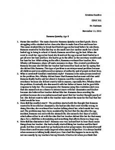
At the end of the top-down traversal, we have a CND proof ϕ of c σ ∗ from S. Since σ ∗ is the global substitution of all substitutions used in ψ 0 and ψ 0 derives κ, we have that c σ ∗ = c. Therefore, ϕ is a CND proof of c from S, as desired. Example 4. To illustrate the transformation of CR derivations into CND derivations used in the proof of Theorem 2, Fig. 8 shows the CND derivation obtained by transforming the CR derivation shown in Fig. 4. Corollary 2. CR is sound. Proof. Let ϕ be an arbitrary CR proof of c from S. Then, by Theorem 2, there is a CND proof of c from S. Since the natural deduction calculus CND is sound, c is entailed by S. Therefore, CR is sound.
7.
Simulation of Splitting
Suppose that a prover refutes the set of clauses S ∪ {Γ1 ∨ . . . ∨ Γk } (where the sets of variables Vi of Γi are mutually disjoint), by splitting it into the k sets S ∪ {Γi } (for 1 ≤ i ≤ k) and finding a Resolution refutation ψi for each set S ∪{Γi }. One way to combine these proofs into a single resolution refutation of S∪{Γ1 ∨. . .∨Γk } would be to use the following recursive method: • For i = 1: construct ψ10 by replacing every leaf occurrence
of Γ1 in ψ1 by Γ1 ∨ . . . ∨ Γk , propagating the added literals downwards and factoring the added literals when possible; then ψ10 is not a refutation, but a derivation of Γ2 ∨ . . . ∨ Γk .
[P (a)]2
¬P (a) ∨ Q Q
[P (b)]1
→E
⊥ ¬1 ¬P (b) I →2I ϕ1 : ¬P (a) ∨ ¬P (b)
[¬P (a)]3 Q
P (z) ∨ Q ∀E P (a) ∨ Q →E
[¬P (a)]3
⊥ ¬3 ϕ2 : P (a) I ϕ2 ϕ1 →E ¬P (b) ¬Q
P (v) ∨ ¬Q ∀E P (b) ∨ ¬Q →E ⊥
ϕ02
¬P (b) ∨ ¬Q →E ¬Q ¬E
P (y) ∨ ¬Q ∀E P (a) ∨ ¬Q →E ¬Q ¬E
¬P (a) ∨ Q →E Q ¬E
where ϕ02 is a reference to a copy of ϕ2 . Figure 8. CND Refutation Simulating the CR Refutation from Fig. 4. 0 • For i from 2 to k: construct ψi+1 by replacing every leaf
occurrence of Γi+1 in ψi+1 by the subproof ψi0 deriving Γi+1 ∨ . . . ∨ Γk ; as before, propagate the added literals downwards 0 and factor them when possible, so that ψi+1 is a proof of Γi+2 ∨ . . . ∨ Γk , if i + 1 < k, or ⊥, otherwise.
However, this method is undesirable, because it requires a substantial modification of the component proofs ψi . The modified subproofs are larger (because of all the additional literals), and this may hinder readability of the proof by humans and reduce the efficiency of automatic proof checking. A pragmatic approach is to disregard the attempt to output a single refutation for the original problem and simply output all the separate proofs for the split problems instead. Keeping track of all splittings is important, particularly in the more general case where splitting is done recursively (i.e. where each set S ∪ {Γi } can be split further). This seems to be the approach taken by most automated theorem provers. Splittings performed during the proof search are recorded in the proof file in an extra-logical way, which may even violate informal semantic requirements of the TPTP proof format7 . In CR, splitting can be simulated in such a way that the refutations for the split sub-problems can be combined without the drawbacks that are incurred when this is done in Resolution. Suppose that ϕi are derivations of S ∪ {Γi }. Then a refutation ϕ of S ∪ {Γ1 ∨ . . . ∨ Γk } can be constructed by combining all the ϕi (for 1 ≤ i ≤ k) using the following recursive method: • For i = 1: construct ϕ01 by replacing every leaf occurrence of i Γ1 in ϕ1 by the following subproof (where `1i , . . . , `n i are duals of the literals in Γi ):
[`12 ]2
...
1 2 [`n 2 ]
...
[`1k ]k Γ1
...
n
[`k k ]k
Γ1 ∨ . . . ∨ Γk
u(ε)
Then construct ϕ01 by adding a conflict-driven clause learning to the bottom of ϕ∗1 : 7 TPTP’s
general proof format (Sutcliffe 2009) requires that the conclusion of an inference rule be a logical consequence of its premises. This limitation prevents an easy representation of natural deduction’s implication introduction rule, tableaux’s β rule or splitting. CR’s conflict-driven clause learning is also affected by this limitation.
• For i from 2 to k: construct ϕ0i by replacing every leaf occur-
rence of Γi in ϕi by the following subproof: .. 0 .. ϕi−1 ⊥ i Γi cl The desired refutation ϕ of S ∪ {Γ1 ∨ . . . ∨ Γk } is taken to be ϕ0k . This method of simulating splitting in CR requires no internal modification of the proofs ϕi : the modified proofs ϕ0i (2 ≤ i ≤ k) are just ϕi with a few cl inferences on top. Hence, there is no loss in readability, and the only overhead for automatic proof checking is caused by the extra need to check the additional cl inferences. If the leaf clause Γi occurs only once8 , a single cl inference suffices, in fact. Therefore, the increase in proof size and the overhead for proof checking are negligible. The simulation described here shows that splitting can be seen as a macro-rule that performs, for a variable-disjoint component Γi , batch decisions assuming the duals of all literals not in Γi . The first-order mechanism of decisions and conflict-drive clause learning provided by CR is, however, more general, because it allows splitting even when the components are not variable-disjoint.
8.
CR with Sequent Notation
The proof of CR’s soundness in Section 6 demonstrates that there is a lot in common between CR and natural deduction. In the same way that natural deduction can be presented with a sequent notation, in which assumptions are listed in the antecedent of the sequent (i.e. at the left side of the turnstile symbol), CR can also be presented with a sequent notation, with decision literals kept at the antecedent. This is shown in Fig. 9. With the sequent notation, it is easier to state the inference rule for conflict-driven clause learning. All the substitutions that should be applied to the literals whose duals will be part of the learned clause have already been applied to the literals in the antecedent. There is no need to look at the substitutions that have been used in the paths above. On the other hand, the presentation with sequent 8 It
may be reused many times, since ϕi does not need to be tree-like.
9.
Decision: `i ` [`]i
Initial: `c if c is an input clause
Unit-Propagating Resolution: ∆1 ` `1
. . . ∆1 ` `n ∆ ` `01 ∨ . . . ∨ `0n ∨ ` u(σ) ∆1 σ, . . . , ∆n σ, ∆ σ ` ` σ
where σ is a unifier of `k and `0k , for all k ∈ {1, . . . , n}.
Conflict: ∆1 ` ` ∆2 ` `0 c(σ) ∆1 σ, ∆2 σ ` ⊥ where σ is a unifier of `k and `0k , for all k ∈ {1, . . . , n}.
Conflict-Driven Clause Learning: 1 n ∆, `i1 σ11 , . . . , `i1 σm , . . . , `in σ1n , . . . , `in σm n 1
`⊥
1 n ∆ ` (`1 σ11 ∨ . . . ∨ `1 σm ) ∨ . . . ∨ (`n σ1n ∨ . . . ∨ `n σm ) n 1
cli
where σjk (for 1 ≤ k ≤ n and 1 ≤ j ≤ mk ) is the composition of all substitutions used on the j-th path from `k to ⊥. Figure 9. CR with Sequent Notation
notation is much more redundant and bureaucratic. Whereas in the standard presentation, the use of decision literals is a powerful way to reduce the size of clauses (as in the simulation of splitting), this beneficial effect is lost in the presentation with the sequent notation, because the decision literals are carried along in the antecedents. For example, if we have the clause ¬`1 ∨ . . . ∨ ¬`n ∨ `, then assuming the duals of the first n literals and resolving them with the clause through unit-propagation would result in the unit clause ` in the standard presentation. With sequent notation, on the other hand, we would obtain `1 , . . . , `n ` `. While this may be conceptually convenient, because it reminds us explicitly that the unit clause ` holds only under the assumptions `1 , . . . , `n , we have no reduction in size if we also count the antecedent’s size. In fact, because the proof may be a non-tree-like DAG, and decision literals may be instantiated by different substitutions along different paths of the DAG, several instances of the decision literal will accumulate in the antecedent. The number of instances may be in the worst case exponential in the height of the derivation. That is one reason why the standard presentation, where the dependence of ` on assumptions and the substitutions used to instantiate the decision literals remain implicit in the derivation, is preferable. This is particularly important during proof search, in which not all inferences are useful and we do not want to apply substitutions and accumulate copies of literals unnecessarily along the derivation. We should do that only when a conflict, warranting conflict-driven clause learning, is reached.
Related Work
The seminal work of Baumgartner and Tinelli (2003; 2014) defining the Model Evolution (ME) procedure was probably the first lifting of DPLL to the first-order case. It was later extended with a lemma learning rule (Baumgartner, Fuchs and Tinelli 2006), while retaining a traditional DPLL flavor (distinct from the conflict graph approach). In model evolution, decision literals do not contain standard variables, but parameters, which are variables with special semantics and behavior in the case of backtracking and clause learning. CR may be considered simpler, because it does not introduce the notion of parameter; however, in contrast to model evolution, for CR the problem of interpreting decision literals as a model has not been investigated yet. More recently, Alagi and Weidenbach (2015) proposed the Non-Redundant Clause Learning (NRCL) procedure generalizing CDCL to the Bernays-Sch¨onfinkel fragment of first-order logic. They introduce the notion of blocked decisions and clauses, which restricts the decisions that can be made and thus allows them to prove that the learned clause is non-redundant (whereas in CR they might not be). They also introduce the notion of constrained literals, which allow more compact representation of the model. In CR, such optimizations and restrictions are intentionally avoided, in favor of a simple calculus focused on the core aspects of generalizing decisions and conflict-driven clause learning to full first-order logic. Bonacina, Fuhrbach and Sofronie-Stokkermans (2015) give a preview of a yet unpublished first-order Semantically-Guided Goal Sensitive (SGGS) procedure inspired by CDCL. As they observe, there is a symmetry between positive and negative literals in the propositional case (i.e. in the sense that when a decision literal ` is false, ` is true) which appears to be lost in the first-order case (i.e. because when ` is false, we cannot conclude that ` is true; we can only conclude that ` σ is true for some σ). One of the main challenges in lifting conflict-driven clause learning to first-order lies precisely in computing and dealing with the substitution σ when a decision literal ` leads to a conflict and a clause containing ` σ must be learned. Instead of addressing this challenge, they circumvent it by introducing the notion of uniform falsity, according to which ` must be true when ` is uniformly false. With this notion, clause learning is still essentially propositional and it is not triggered at every conflict (in the standard non-uniform sense of conflict). For instance, a conflict between R(x) and ¬R(b) does not lead to clause learning but must be repaired by revising R(x) to x 6= b . R(x) instead. The variety of approaches attempting to generalize CDCL to first-order logic shows that this is not a trivial task. The most pragmatically successful approaches so far have harnessed the power of SAT-solvers in first-order (or even higher-order) logic not by generalizing their underlying procedures but simply by employing them as black-boxes inside a theorem prover (Korovin 2008; Voronkov 2014; Brown 2012).
10.
Conclusion
The development of the Conflict Resolution calculus CR was initially motivated by the recent success of CDCL and by the desire to generalize its main ideas to first-order logic. However, CR can also be seen as the convergence of two ideas that actually precede CDCL by several decades. The first one is the assumption mechanism introduced by Gentzen (1935) in his natural deduction calculus. The second one is Robinson’s generalization of the resolution rule to first-order logic through unification (1960). CR extends resolution as natural deduction extends Hilbert-style proof systems: decision literals are essentially assumptions, and conflict driven clause learning corresponds to (several applications of) nat-
ural deduction’s implication introduction rule. And whereas Robinson used unification to generalize resolution, CR uses unification to generalize conflict-driven clause learning. From a historical perspective, what we are seeing today is similar to what happened between 1960 and 1965. In 1960, Davis and Putnam defined the propositional resolution rule, which can be regarded as an efficient machine-oriented variant of modus ponens (implication elimination). The first-order case was then handled by grounding/instantiating the first-order problem and using the propositional resolution rule. In 1965, Robinson’s direct generalization of the resolution rule to the first-order case enabled a breakthrough in first-order automated theorem proving. Nowadays, we have a powerful propositional conflict driven clause learning rule, which can be regarded as an efficient machine-oriented variant of implication introduction. The first-order case is being handled by essentially grounding/instantiating the problem in various ways and using the propositional rule. If history repeats itself, we might see another breakthrough when clause learning is directly lifted to the first-order case through unification, as done in the CR calculus proposed here. A well-defined proof system is just a first step towards the development of a proof search procedure that could be implemented as an efficient theorem prover. There is much more to the efficiency of a modern SAT-solver than just the ideas of decision literals, conflict-driven clause learning and unit-propagation. SATsolvers use restarts, strategies for selecting decision literals and data-structures that allow efficient unit-propagation, fast conflict graph analysis and fast backtracking. Adapting these proof search strategies and implementation techniques to the Conflict Resolution calculus CR is beyond the scope of this paper, but is a crucial direction for future work. Acknowledgements: Bruno is grateful to Pascal Fontaine, who supervised him during his first post-doc, providing a great opportunity for him to learn some of the essential ideas behind current SAT-solvers. Bruno is thankful to Peter Baumgartner, who shared his experience in model evolution and other related methods, when they discussed the idea of CR in May 2015. Bruno would also like to thank Hans de Nivelle and Jens Otten for discussions during the Vienna Summer of Logic about limitations of the TPTP proof format that affect the representation of natural deduction and tableau proofs.
References Gabor Alagi and Christoph Weidenbach. “Non-Redundant Clause Learning”. In: FroCoS (2015), pp. 69–84. Evert W. Beth. “Semantic Entailment and Formal Derivability”. In: Mededelingen van de Koninklijke Nederlandse Akademie van Wetenschappen, Afdeling Letterkunde 18.13 (1955), pp. 309–342.
Maria Paola Bonacina, Ulrich Fuhrbach and Viorica Sofronie-Stokkermans. “On First-Order Model-Based Reasoning”. In: Logic, Rewriting and Concurrency (2015), pp. 181–204. Chad E. Brown. “Satallax: An Automatic Higher-Order Prover”. In: IJCAR (2012), pp. 111–117. Chad E. Brown. “Reducing Higher-Order Theorem Proving to a Sequence of SAT Problems”. In: Journal of Automated Reasoning (2013), pp. 57–77. Martin Davis and Hilary Putnam. “A Computing Procedure for Quantification Theory”. In: Journal of the ACM 7 (1960), pp. 201–215. Martin Davis, George Logemann and Donald Loveland. “A Machine Program for Theorem Proving”. In: Communications of the ACM 5(7) (1962), pp. 394–397. Gerhard Gentzen. “Untersuchungen u¨ ber das logische Schließen I & II”. In: Mathematische Zeitschrift 39.1 (1935), pp. 176–210 & 405–431. Konstantin Korovin. “iProver - An Instantiation-Based Theorem Prover for First-Order Logic (System Description)”. In: International Joint Conference on Automated Reasoning (IJCAR) (2008), pp. 292–298. Joao Marques-Silva and K.A. Sakallah. “GRASP: A New Search Algorithm for Satisfiability”. In: International Conference on Computer-Aided Design (1996), pp. 220 – 227. Joao Marques-Silva, Ines Lynce and Sharad Malik. “Conflict-Driven Clause Learning SAT Solvers”. In: Handbook of Satisfiability (2008), pp. 127 – 149. J. McCharen, R. Overbeek and L. Wos. “Complexity and Related Enhancements for Automated Theorem-Proving Programs”. In: Computers and Mathematics with Applications 2 (1976), pp. 1–16. W. McCune. “Prover9Manual” (2006). Alexandre Riazanov and Andrei Voronkov. “The Design and Implementation of VAMPIRE”. In: AI Communications 15(2-3)(2002), pp. 91–110. John Alan Robinson. “A Machine-Oriented Logic Based on the Resolution Principle”. In: Journal of the ACM 12.1 (1965), pp. 23–41. George Robinson and Larry Wos. “Paramodulation and Theorem-Proving in First-Order Thories with Equality”. In: Machine Intelligence 4 (1969), pp. 135–150. Stephan Schultz. “System Description: E 1.8”. In: LPAR (2013), pp. 735– 743. Geoff Sutcliffe. “The TPTP Problem Library and Associated Infrastructure: The FOF and CNF Parts, v3.5.0”. In: Journal of Automated Reasoning 43.4 (2009), pp. 337–362. Andrei Voronkov. “AVATAR: The Architecture for First-Order Theorem Provers”. In: CAV (2014), pp. 696–710. Uwe Waldmann. “Superposition”. In: Encyclopedia of Proof Systems (2015). Uwe Waldmann. “Saturation with Redundancy”. In: Encyclopedia of Proof Systems (2015).
Leo Bachmair and Harald Ganzinger. “Completion of First-Order Clauses with Equality by Strict Superposition (Extended Abstract)”. In: 2nd International Workshop Conditional and Typed Rewriting Systems, LNCS 516, Springer (1990), pp. 162–180.
Christoph Weidenbach. “Combining Superposition, Sorts and Splitting”. In: Handbook of Automated Reasoning (2001), pp. 1965–2013.
Leo Bachmair and Harald Ganzinger. “Rewrite-based Equational Theorem Proving with Selection and Simplification”. In: Journal of Logic and Computation 4.3 (1994), pp. 217–247.
Christoph Weidenbach, Dilyana Dimova, Arnaud Fietzke, Rohit Kumar, Martin Suda, Patrick Wischnewski. “SPASS Version 3.5”. In: CADE (2009), pp. 140–145.
Peter Baumgartner. “Model Evolution Based Theorem Proving”. In: IEEE Inteligent Systems 29(1) (2014), pp. 4–10.
Nathan Wetzler, Marijn Heule and Warren A. Hunt Jr. “DRAT-trim: Efficient Checking and Trimming Using Expressive Clausal Proofs”. In: SAT (2014), pp. 422–429.
Peter Baumgartner and Cesare Tinelli. “The Model Evolution Calculus”. In: CADE (2003), pp. 350–364. Peter Baumgartner, Alexander Fuchs and Cesare Tinelli. “Lemma Learning in the Model Evolution Calculus”. In: LPAR (2006), pp. 572–586. Armin Biere. “Picosat Essentials”. In: Journal on Satisfiability, Boolean Modelling and Computation (JSAT) (2008).
Christoph Weidenbach. “The Theory of SPASS Version 2.0”. In: SPASS 2.0 Documentation.
Lintao Zhang, Conor F. Madigan, Matthew H. Moskewicz, Sharad Malik. “Efficient Conflict Driven Learning in a Boolean Satisfiability Solver”. In: International Conference on Computer-Aided Design (2001), pp. 279–285.
Appendix - A Standard Non-Clausal Classical Natural Deduction Calculus A standard natural deduction calculus for minimal quantified logic extended with a classical rule for double negation elimination is shown in Fig. 10. Implication Elimination (Modus Ponens): A
A→B → E B
Implication Introduction: [A]i .. .. B →iI A→B Universal Quantification Elimination: A ∀E A{x\t} Universal Quantification Introduction: A{x\α} ∀I A α must be an eigen-variable: it should occur neither in Γ nor in any undischarged assumption. Double Negation Elimination: (A → ⊥) → ⊥ ¬˙ ¬˙ E A Figure 10. A Non-Clausal Natural Deduction Calculus