Confluently Persistent Deques via Data Structural Bootstrapping

Chapter

Confluently

Persistent Adam

Deques via Data Structural Robert

L. Buchsbaum*

Abstract We introduce design data

data structural bootstrapping, a technique to structures recursively, and use it to design

confluently persistent deques. Our data structure requires O(log* k) amortized time and space per deletion, where k is the total number of deque operations, tized time for other operations. This result of Driscoll, Sleator, and Tarjan.

1

and constant amorimproves a previous

Introduction

Consider the following operations to be performed nondestructively on linear lists X = (~1, . . . , GE,) and Y = (Yl,...,Ym>: mnkedeque(d)

Return a new list of one element, d.

POP(X)

Return pair (~1, (~2,. . . , z,)).

eject(X)

Return pair (z,, (~1,. . .,2,-r)).

cntennte(X,

Y) Return list (21,. . . , zn,yi,. . . , ym). X may be the same list as Y. Knuth [21] calls such lists deques (for doubleended queues) since access is provided to both ends of the lists. The familiar push and inject operations, which insert elements into the front and rear of lists, are subsumed by catenate. We can also allow separate first(X) and last(X) operations which simply return the first and last elements of list X without creating new lists. While the above operations can all be implemented destructively in 0( 1) worst-case time using doublylinked lists [32], providing a non-destructive implementation is more problematic. By non-destructive we mean that the operations pop, eject, and catenate leave their argument lists wholly unchanged. This falls within the *Dept. of Computer Science, Princeton, [email protected]. Supported by a Fannie and John Hertz Foundation fellowship, NSF Grant No. CCR-8920505, and the Center for Discrete Mathematics and Theoretical Computer Science (DIMACS) under NSF-STC88-09648. tDept.

Institute,

of Computer

Science,

[email protected].

supported by NSF N00014-91-J-1463,

Princeton,

18

NEC

Research

Research at Princeton

and

partially

Grant No. CCR-8920505, ONR Contract and DIMACS under NSF-STC88-09648.

No.

155

Bootstrapping

E. Tarjant

realm of persistent data structures, which we discuss in Section 1.1. Driscoll, Sleator, and Tarjan [17] give a solution to the non-destructive output-restricted deque problem (no eject operation) that runs in O(1) amortized time [33] and space for all the operations except catenate; catenate consumes O(log log k) amortized time and space per operation, where k is the number of operations preceding the catenate. We report a solution to the above problem in which pop and eject require O(log* k) amortized time and space, where k is the number of deque operations performed so far, and all the other operations require O(1) amortized time and space each. Noting that the Driscoll, Sleator, and Tarjan [17] solution to the output-restricted deque problem provides non-constant resource bounds for catenate rather than pop and eject, we can modify our data structure to solve the output-restricted deque problem so that catenate requires O(log(‘) k) amortized time and space, where i is any desired constant, and the other operations take O(1) amortized time and space. The main technique we employ is data structural We use two types of bootstrapping. First, bootstrapping. we abstract fully persistent lists (see Section 1.1) so that their elements are not atomic but rather represent other lists. Second, we implement deques of n elements by recursively decomposing them into collections of deques of O(log n) elements. The first type of bootstrapping, which we call structural abstraction, is used in [17] to implement persistent catenable lists ,using fully persistent (non-catenable) lists and by Buchsbaum, Sundar, and Tarjan [6] to implement catenable heap-ordered deques using non-catenable heap-ordered deques. It is similar to a technique used by Kosaraju [22] in designing catenable deques by dissecting them and storing contiguous pieces on stacks. The second type of bootstrapping, which we call structural decomposition, is similar to an idea of Dietz [lo], who recursively decomposes indexed 2-3 trees so that their leaves store smaller indexed 2-3 trees, improving their performance from O(logn) to O(log* n) amortized time. Structural decomposition differs from ideas used to solve decomposable search problems [5] and from other ad hoc instances of data structure decomposition

156

BUCHSBAUM

(e.g., [12, 13, 14, 35, 37, 381) in that these previous results do not use recursive decomposition. Non-destructive (or, in the parlance of Section 1.1, conj7uently persistent) deques have many uses in highlevel programming languages such as LISP, ML, Scheme, etc. [31], in which side-effect-free list operations are fundamental. They also can be used in the implementation of continuation passing in functional programming languages [4]. Furthermore, our results impact the study of persistent data structures. 1.1 Persistent Data Structures Data structures normally provide two types of operations: queries and updates. In the terminology of [16], a data structure is ephemeral if an update destroys the version of the data structure being changed; i.e., there is always one and only one valid version. A data structure that allows queries but not updates to previous versions is partially persistent; in this scheme, one thinks of a time-line of versions. Allowing previous versions to be updated yields a fully persistent data structure and produces a tree-like notion of time. There has been much previous work on making various data structures partially or fully persistent [7, 9, 15, 20, 23, 24, 25, 26, 291. There have also been some results providing general methods for making entire classes of data structures persistent [ll, 13, 16, 27, 301. In particular, Driscoll et al. [16] show how many pointer-based data structures may be made partially or fully persistent with only a constant factor overhead in time consumption and using only a constant amount of space per persistent update; both bounds are amortized. Their result is subject to the important restriction that any node in the ephemeral data structure may have only a fixed number of incoming and outgoing pointers. Dietz [l l] makes arrays fully persistent so that access and store operations on an array of size n require O(log log n) time (amortized expected for store) and linear total space. None of these previous results, however, allows updates involving more than one version; combining two versions, as is done in deque catenation, is not possible. This type of update leads to a DAG-like concept of time, and a data structure in this setting is called confluently persistent in [17]. Driscoll et al. [16] leave open solving this problem in general. While we do not offer such a general solution, to date we are aware of only [17] as a previous result in this direction. Our work provides an asymptotically more efficient solution to a more general problem. Further, we demonstrate the power of data structural bootstrapping as a tool for designing highlevel data structures. We begin by presenting a data structure in which all operations require O(c“‘z’ ‘) amortized time and space, for some constant c. While c’“s*k seems to be an unusual function, it results from a natural recurrence:

AND

bc

TARJAN

gh

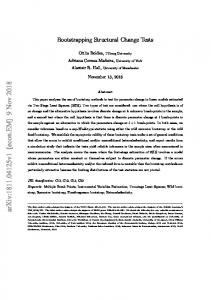
Figure 1: (a) Linking two trees; (b) After deleting the leftmost leaf of the linked tree of (a); (c) After deleting the leftmost leaf of the tree of(b).

F(n) = c’F(logn) + O(1). This recurrence arises from the structural decomposition of a deque of n elements into a collection of deques of O(log n) elements each. Section 2 describes the deque tree, a tree whose leaves represent a deque, and discusses a way to keep it balanced. Section 3 demonstrates how to implement deque trees using only lists and catenable deques. While [17] suggests a similar decomposition of trees into paths which in turn are represented by trees, we observe that a decomposition of trees into paths accessible only at their ends is possible and preferable. Section 4 then introduces the two kinds of data structural bootstrapping. The first kind, structural abstraction, abstracts fully persistent lists so that their elements contain version numbers “pointing to” confluently persistent deques, which in turn are abstracted so that their elements contain version numbers pointing to other fully persistent lists. The second kind, structural decomposition, uses the properties of the deque trees to show that O(logn)-sized confluently persistent deques suffice to implement n-sized confluently persistent deque trees via the above method. We then improve our data structure in Section 5 to reduce the resource bounds for pop and eject to O(log* k) each and those for the other operations to O(1) each. 2

Deque

Trees

Consider an ordered tree [21] embedded in the plane with the root at the top and the leaves at the bottom. We exploit the induced left-to-right order of the leaves of the tree to make the tree represent a list. The two operations we perform on the tree are link, which makes the root of one tree the new leftmost or rightmost child of the root of another (see Figure la), and delete, which removes

DATA STRUCTURALBOOTSTRAPPING

157

either the leftmost or the rightmost leaf of the tree (see Figure lb). Link corresponds to deque catenation, and delete corresponds to pop and eject. The internal nodes of the tree can be of arbitrarily high degree, but we make sure that they are at least binary; to do so requires replacing an internal node x by its remaining child if a deletion renders z unary. See Figure lc. It also requires a special case of link when linking two single-node trees; in this case, a new root node is created with the two old nodes becoming its children. Since delete preserves the left-to-right order of the remaining leaves, such trees can be used to implement catenable deques, and we therefore call them deque trees. The remainder of this section describes how to keep deque trees “in balance.” The next two sections describe a method to implement confluently persistent deque trees (and thus deques). The efficiency of the implementation derives from the deque tree balance property. We define a pull operation on deque trees just as [17] defines this operation on similar trees; [6] defines a slightly different form of pull. Let z be the leftmost non-leaf child of the root T of a tree T, and let x’ be the leftmost child of Z. A pull on T cuts the link from x’ to x and makes x’ a new child of r just to the left of x. Additionally, if x is now unary, it is replaced by its remaining child. See Figure 2. Pull preserves the left-to-right order of the leaves of T. We call a tree fiat if all the children of the root are leaves or if the tree is a singleton node. A pull on a flat tree does nothing. A pull on a non-flat tree increases the degree of the root by one. In what follows, the size of a tree T, denoted by ITI, is the number of leaves in T. We now describe how to use pulls to keep deque trees balanced, i.e., of logarithmic depth. We define the depth of a deque tree to be the length of its longest root-to-leaf path. Denoting the depth of a deque tree T by dT, we maintain the invariant that ITI 2 cdT for some constant c > 1. To do so, we perform h pulls on T for each deletion on T, for some constant le. Also, we implement linking by size; i.e., when linking two trees A and B, we link the one with fewer leaves to the one with more, breaking a tie arbitrarily. This technique is also used to maintain balanced trees in the disjoint set union problem [34].

LEMMA 2.1. If k > 2 then a non-root node in a deque tree never becomes a root node of a deque tree T unless T is a singleton node. PROOF: New root nodes are created by the

make-

deque operation and by linking two singleton trees together. Consider when a root node T of some tree becomes a non-root node due to a link. Assume at some point in the future that T becomes a root node of some tree X. Now consider the most recent tree S formed before X by linking a tree R containing r to another tree R’. Let T’ be the root of R’ (and thus of S), and note that (R’J 2 (RI. By this definition, T’ never becomes a

non-root node before X is created, but, it may acquire new children as a result of future links. Denote by T the evolving tree rooted at T’, initially S, as leaves are deleted from it and other trees linked to it. Let a total of x leaves be added to T via links after the formation of S. For r to become a root node, all the leaves of R’ plus all these x leaves must first be deleted from T, resulting in k( IR’I + x) pulls being applied to T. If k >_ 2, then this is sufficient to flatten T, since each pull increases the degree of the root of T by one, and there are always more pulls remaining than leaves of T. If r is a non-root internal node in a tree which is flattened, then r is removed during this process. Therefore, for T to be flat and still contain r, T must be a leaf. For T to become a root, all the other leaves of T must first be deleted, leaving the single node T as tree X. 0

THEOREM2.2. If 1

< c < 2 and k >

A,

then

ITI 2 cdT.

PROOF: We proceed by induction on the number of deque tree operations. A singleton tree of depth 0 is created by makedeque. Consider any depth-increasing link of a tree T to a tree T’ yielding tree T”. We have 11= dT + 1 > dT#. By induction, ITI > cdT. Linking $ size gives IT’/ 2 ITI and thus IT”1 2 2cd~. As long as c 5 2, the invariant iolds. Assume some deletion creates a tree X with root, r Let such that 1x1 < cdx. We derive a contradiction. R be the most, recent tree rooted at T formed before X by a depth-increasing link. By the above analysis of linking, we know that IR] = 2cd~-’ + x for some x >_ 0. The intermixed sequence of deletions and links that produces X from R cannot make r a non-root node; otherwise Lemma 2.1 shows that X is the singleton node T. Let T be the evolving tree, initially R, rooted at T as leaves are deleted from it and other trees linked to it. For 1x1 < cdx to be true, at least (2 - c)cdRT1 +x + y leaves must be deleted from T, where y is the total number of leaves added to T via links. If k 2 &, then, as in the proof of Lemma 2.1, T is flattened, and the depth invariant holds until the next depth-increasing link. So no depth violation occurs. Cl In particular, we can set c = 3/2 and k = 4. COROLLARY2.3. If T is a deque tree, then dT =

O(logIW 3

Decomposition

into

Spines

Here we describe how to decompose a deque tree into a collection of spines. We define spines bottom up. A left (right) spine of a tree is a maximal tree path (x0, . . . , Q), such that x0 is a leaf and xi is the leftmost (rightmost) child of xi+1 for 0 5 i < 1; we say the spine terminates or ends at xl. We represent a deque tree as a set of spines so that all the deque tree operations require accessing the spines only at their ends. By recursively representing the

158

BUCHSBAUM

b

c

g

h

b

c

g

h

AND TARJAN

g

h

Figure 2: Two pulls applied to a tree. spines by smaller deque trees, we obtain a bootstrapped implementation of confluently persistent deques. Recall the deque operations from Section 1. We first describe how to implement them ephemerally using deque trees. Later we show how to make the implementation persistent. Let root(T) be the root of a deque tree T. We store the left and right spines terminating at root(T) in the deques Is(T) and rs(T); these are called the root spines. For a node x with i children in T, let the children of x be cb, . . . , CL in left-to-right order. Let 1; (ri) be the left (right) spine terminating at ci for 1 5 j < i. We store at node x a pointer to a doubly-linked list s-list(z) whose elements left-tori-l 1’. i.e ., we record the right are r15) l2I, r2$?a”‘> ii-1 z > I j ZY right spine terminating at z’s leftmost child, the left and right spines at its middle children, and the left spine at its rightmost child. The “missing” spines are recorded in the s-lists of some other nodes (if they are not the root spines). All the spines are stored as deques with the leaves at the front (pop) ends. The spine deques, therefore, contain as elements nodes pointing to their respective s-lists. See Figure 3. A node in a deque tree is thus stored in precisely two spines, appearing as the top node in at least one of them. The operations on the s-lists are (1) insert(1, 2, y) insert y after x in s-list 1; and (2) delete(1, cc) - delete x from s-list 1 and return x. Additionally, each element x in an s-list has a pred(c) and succ(c) pointing to the predecessor and successor of z respectively. Special sentinels head(l) and tail(l) point to the first and last elements of s-list 1, and the special case insert(1, pred(head(l)), x) inserts a new first element x into 1. To make a new deque tree T with one node x, we set Is(T) and rs(T) to be the singleton deque (x) and s-list(c) to be 8. Now we describe how to link a deque tree A to another deque tree B. If A and B are both singleton deque trees, we create a new structure for the resulting tree. Otherwise, we make root(A) the new leftmost child of root(B); the other case is symmetric. First, eject root(B) from Is(B) and insert the new Is(B) as the new head of s-list(root(B)); this is now the left spine terminating at the new second-leftmost child of B. Then insert m(A) as the new head of s-list(root(B)); this is now the right spine terminating at the new leftmost child

Figure 3: A subtree rooted at node x and a portion of its spine decomposition structure. Boxes surround spine deques, and s-lists are bracketed; li (ri) refers to the spine deque for the left (right) spine terminating at the root of subtree Ti. Null s-lists (for leaves) are omitted.

of B. Finally, reset Is(B) to be the catenation of Is(A) and root(B). A deletion involves more steps, so we merely give pseudocode for deletion. See Figure 4. The code in Figure 4 is for a deletion of the leftmost leaf of T; the code for deletion of the rightmost leaf is symmetric. It is crucial that the nodes not store the first left spine or the last right spine; these are stored as parts of other, bigger spines. This lack of duplication allows the implementation of the deque tree operations by simple deque and s-list operations. It is also critical that the internal nodes remain at least binary; this avoids the situation in which two spines intersect at more than one node. To implement pulls, we augment the s-lists to store as secondary information doubly-linked lists of pointers to the non-leaf children of each node. Each node also stores its degree. Using the notation above, if 4 is a non-leaf child, then a pointer points to 1; in s-list(x); the exception is that if CL is a non-leaf child, then the

DATA STRUCTURAL

BOOTSTRAPPING

(2, Is(T)) + pop(ls(T)) // the leftmost leaf of T (Y, W)) +- pop(ls(T)) // z’s parent if (y has more than 2 children) then delete(s-list(y), head(s-l&(y))) // discard 2 as the // old right spine 1 + delete(s-M(y), head(s-M(y))) // next // left spine Is(T) .+ catenate(l, catenate(makedeque(y), Is(T))) else if (y # root(T)) then // must delete y and promote // other child (s, WY)

+- POP(W))

// Y’S parent

1 + taiI(s-l&(y)) // next left spine r + delete(s-M(g), head(s-list(g))) // right spine // terminating at y (y, r) c eject(r) // remove y insery;-l;;.s;);flred(head(s-l&(g))), T) // new Is(T) t’~ate~a~$, catenate(makedeque(g), Is(T))) else // y = root(T) and has two children Is(T) t tail(s-list(y)) // new left spine of T (y, rs(T)) + eject(rs(T)) // delete y

Figure 4: Pseudocode for deletion of leftmost leaf of T. Double slash (//) precedes comments.

pointer points to Y:. This seems unfortunate, but we must handle the case of a pull affecting a root spine slightly differently from one affecting a middle child of root(T) anyway. It is straightforward to maintain this secondary information when modifying the s-lists, and for clarity we omit this part of the implementation from the description. We merely mention that this is possible since actual s-list modifications only take place at either the ends of the s-lists or near elements in the s-lists which are .themselves targets of these secondary pointers. For brevity, we omit the pseudocode to perform the pull operation. We simply note that a pull, like a deletion, requires a constant number of operations on spine deques and s-lists. The above explanation shows that a constant number of ephemeral deque and s-list operations suffice to implement any ephemeral deque tree operation. Next we describe how to use the spine decomposition of deque trees to implement confluently persistent deques. 4

Data

Structural

Bootstrapping

Section 3 shows how to implement ephemeral deque trees using catenable deques and s-lists. We now describe how to implement confluently persistent deque trees. We use an idea of [17] to bootstrap confluently persistent deques and fully persistent s-lists. First, note that the s-list structure is a bounded indegree structure, in the terminology of [IS]. Further, each

159 s-list(x) has only four access pointers, i.e., entry points to the s-list where access can start. These four points are the two ends and the nodes corresponding to the leftmost and rightmost non-leaf children of Z. Thus, we can use the methods of [16] to make s-lists fully persistent so that a non-destructive s-list operation takes O(1) amortized time and space. For now, assume the existence of confluently persistent deques.

The bootstrapping idea of [17] is to make each element in a persistent s-list point to its respective spine via a version number referring to the corresponding persistent deque. Similarly, each element of a persistent deque contains the version number of the corresponding node’s persistent s-list. We call this structural abstraction. The confluently persistent deque tree T is then fully described by the version numbers of Is(T) and rs(T). We mention that the cases in the above implementation in which a node is popped off a spine only to be recatenated to the spine are present to record the new version number of the node being recatenated to the spine. One implementation detail remains: Updating a spine deque creates a new version of that deque which must be stored in any s-list pointing to the spine; this creates a new version of the s-list, which must be reflected in a “higher” spine pointing to the list, and so on. This is further complicated by the fact that a node occurs in two spines, and when an s-list changes, both copies of the node that points to it must be updated. We fix the second problem by storing the version number of any s-list(x) only in the copy of node x that occurs in the middle of a spine; the copy occurring at the top of a spine is left blank. If both copies occur at the tops of spines, one is chosen arbitrarily to store the version number of s-list(x). This works for the following reason: Any time an s-list(c) is accessed via the copy of node x occurring at the top of a spine, then the spine is either a root spine or a spine actually pointed to by s-list(r) where r is the root of a tree. In either case, both copies of z are readily available via a constant number of deque and s-list operations and so the version number of s-list(x) may be retrieved. No reverse pointers are needed, keeping the number of access pointers small and preserving the validity of the methods of [16]. Now note that any modifications to spines and s-lists occur close to a root spine. I.e., updating a spine might cause an update to an s-list, but the node pointing to this s-list will be on Is(T) or rs(T). Therefore, no cascading sequence of version updates occurs. As an aside, we note that Driscoll, Sleator, and Tarjan [17] use the pull operation to ensure that any modifications to their structure occur close to the roots of their trees, thereby keeping cascading sequences of updates short. While it is clear that s-lists can be made fully persistent using previously known techniques [16], the method described above relies upon the existence of confluently

160

BUCHSBAUM AND TARJAN

persistent deques in their own implementation. Note that to represent a confluently persistent deque of size n, however, we need only be able to implement confluently persistent deques of size O(logn); this is due to Corollary 2.3. This is the second type of bootstrapping we employ: namely, decomposition of a data structure into smaller pieces represented in the same fashion (and some auxiliary data structures, in this case the s-lists). We call this structural decomposition. THEOREM 4.1. Any operation on a confluent/y persistent deque of size n can be performed in O(c”g*“) amortized time and space for some constant c. PROOF: We represent small confluently persistent deques, say of four or fewer elements, by doubly-linked lists. Operations on such a small deque are performed by copying the entire deque and modifying the new copy. Any time a deque increases to a size above this threshold, we implement it via spine decomposition. An operation on a confluently persistent deque tree of n leaves implemented via spine decomposition requires 0( 1) fully persistent s-list operations, each taking O(1) amortized time and space [16]. It also requires O(1) operations on confluently persistent deques that by Corollary 2.3 are of size O(logn). Therefore, for some constants cl and c2, the amortized time and space required by an operation on a confluently persistent deque of size II is F(n), where

F(n) = { P,$ilog n) + O(1)

i: Z ,I Zi

This recurrence is solved by F(n) = O(&‘z* “) for some c.onstant c. 0 We note that confluently persistent deques support “self-catenation,” i.e., forming a new deque by catenating an old one to itself. Therefore, k catenations can generate a deque of size 2”. This potential size explosion is addressed in [17] by a “guessing trick,” which involves guessing how many operations will be performed and keeping the lists truncated to an appropriate size, doubling or squaring the guess and rebuilding the lists each time the number of operations exceeds the previous guess. This technique is important in this previous work, since the resource bounds obtained there of O(log n) and O(loglogn) would otherwise become O(lc) and O(log k) respectively, poor amortized results. Our method requires no such additional machinery, however: Since c is constant, for n = O(2k) we have clog* n = O(c”‘g* k). We conclude this section by mentioning how to improve the performance of catenate, first, and last. The latter two operations can easily be made to take O(1) worst case time by storing with each deque its actual first and last elements. We improve catenate as follows. Treat the root spines (Is(T) and rs(T)) specially by not storing the actual node root(T) in them. We can

now implement the standard push and inject operations by directly modifying the spine decomposition structure of the affected deque tree using only s-list operations, rather than calling catenate. Now use push and inject in place of catenate wherever possible in the implementation. By doing all this, we remove the eject call from the link operation and catenate becomes a non-recursive call, utilizing only a constant number of inject and slist operations and thus taking O(1) amortized time and space per call. In the next section, we shall reduce the cost of deletion to O(log* k) amortized time and space. 5

Improving

the

Data

Structure

The only non-constant-cost operation in our data structure is deletion. A deletion on a deque of size n requires a number of deletions on deques of size O(logn), yielding an O(c log* n ) bound. Here we modify our data structure so that a deletion from an n-sized deque requires at most one deletion from an O(log n)-sized deque, thereby reducing our resource bound to O(log* n). For clarity, we use the term deletion to refer to the corresponding operation on a deque of n items or a deque tree of n leaves, and we use subdeletion to refer to the operation on a smaller (O(logn)-sized) structure. In our original implementation, one deletion can require four subdeletions to modify the spine decomposition of the deque tree plus some number of pulls, each of which potentially requires three subdeletions. In Section 5.1, we modify the representation of the spine decomposition to reduce to one the number of subdeletions required to update the spine decomposition of a deque tree undergoing a deletion. In Sections 5.2 and 5.3 we eliminate the pulls altogether and replace them with another mechanism to maintain balanced deque trees. Section 5.4 then provides the details on how to make the new implementation persistent. 5.1 Modified Representation As previously mentioned, the present implementation can require as many as four subdeletions per deletion in order to update the spine decomposition of the deque tree: (1) to remove 2, the node being deleted, (2) to remove or update y, Z’S parent, (3) to update y’s parent, say g, and (4) to remove the terminating node (y) of the right spine terminating at g’s leftmost child. Our new implementation eliminates the first three of these deletions. We keep the same spine decomposition described in Section 3; i.e., the root spines and s-lists still record the same spines as before. We increase the degree invariant maintained at each non-root internal node so that each such node now has degree at least three; the root node still has degree at least two. Our biggest change, though, is how we store the spines. Whereas before each spine was stored as a deque, we now store the leaf and terminating nodes of each spine separately and keep only

DATA STRUCTURAL BOOTSTRAPPING

Figure 5: A deque tree T. Dashed lines are paths of nodes that comprise middle deques of spines; triangles represent other subtrees descending from the nodes. The first element of the deque is 21 = leuf(ls(T)); y = first(deq(ls(T))) is 21’s parent in T, and g = second(deq(ls(T))) is y’s parent in T. Let 1 = succ(head(s&$y))); 1 is the left spine terminating at y’s second child ~1. Then zs = leaf(/) is the second element of the deque. We can change xi and x2 in place in T in O(1) time.

the non-leaf and non-terminating (middle) nodes of the spine in a deque. Here we investigate the impact of the modifications on the algorithm for maintaining the spine decomposition. Given any spine s, leaf(s), den(s), and 2enn(s) respectively give us the leaf node, middle deque, and terminating node of s. First, we no longer need to maintain the first and last elements of each deque, since we can access these and leuf(rs(T)) each in O(1) elements as leuf(ls(T)) time. Additionally, we can now change in place the first and second (and last and second-to-last) elements of any deque; that is, we can modify them without performing subdeletions on the spines of T. To change the first element in place merely requires updating leaf(ls(T)). To change the second element in place, we first access y = leuf( deq (Is(T))); this is the parent of leaf(ls(T)) in T. We then take from s-list(y) the left spine 1 terminating at y’s second child. The second element of T is leaf(l), and we can modify this directly. This produces a new’ left spine 1’ which we store in the proper place in s-list(y). In a persistent setting, we now have a new version of y, which we can store in Is(T) by changing y = first (deq(ls(T))) in pl ace; of course, we also have a new version of Is(T). See Figure 5. Changing the

161 last and second-to-last elements of a deque is symmetric. By the same reasoning, we can also use second(T) and second-to-lust(T) to access the second and secondto-last elements of a deque in O(1) time. We exploit the new representation of a spine and changing in place to remove the three deletions cited above. This is best illustrated when we have to delete y to prevent its degree from falling below three. Let z1 and zs be y’s middle and rightmost children, respectively. Note that y is the terminating node of the right spine terminating at g’s leftmost child (y). We eject ts from that spine’s middle deque; 2s becomes the new terminating node. We also have to change g in place to reflect the changes to s-list(g): the replacement of the right spine ending at g’s leftmost child and the addition of the left spine terminating at zs and the right spine terminating at zi. As zi is the terminating node of the left spine ending at y’s second-leftmost child, we replace The new section of y with z1 in place in deq(ls(T)). Is(T) comes from the leaf node and middle deque of the left spine terminating at tl , and we can catenate the appropriate segments. In fact, this case is the only time a subdeletion occurs. If y remains on the spine, then no subdeletions occur. Note that the higher degree invariant slightly complicates linking deque trees: If the root of the smaller tree being linked has degree two, then we must make each of its children a child of the root of the larger tree rather than link roots. For brevity, we omit the pseudocode showing the new procedures. There are a couple of special cases to be addressed. First, in the above case (where y is replaced by zi), if ~1 is a leaf node then we would have to pop y from deq(ls(T)), for in this case .zl would become leaf(ls(T)). To avoid this second subdeletion, we instead replace y in place with 22, catenate the middle deque of the left spine terminating at a2 to deq(Zs(T)), and add z1 as the new leftmost child root(T); this last step is just a push. ;’ rzkis;r a leaf, then we do the pop from deq(ls(T)) ma in = first(Zs(T))), but no eject from the right spine terminating at y is necessary. So, again, only one subdeletion occurs. The second special case is when a spine has fewer than three elements and thus cannot support the new spine representation. In this case, all the operations on the spine can be accomplished by dealing with the elements themselves. 5.2 Deque Traversal Here we introduce the notion of traversing a deque and show how our modified representation facilitates such an action. In Section 5.3, we use deque traversal to help eliminate the pulls. A deque traversal is a sequence of steps that makes available the elements of the deque in head-to-tail or tailto-head order. A deque tree traversal makes available the leaves of the deque tree in left-to-right or right-toleft order. To traverse a deque implemented via spine

162

BUCHSBAUM

decomposition, we need to traverse its deque tree, which involves traversing the smaller deques that make up its spines, and so on. Ephemeral deques allow traversal in O(1) time per element. With our original data structure, it is not clear that this is possible. Our modified representation, however, makes it possible. We traverse the deque tree in symmetric, i.e., depthfirst left-to-right (or right-to-left), order. To visit the leftmost or rightmost child of a node requires performing some part of the traversal of the corresponding spine deque. Visiting a middle child of a node requires accessing the node’s s-list (left-to-right or right-to-left) to obtain and begin traversing the appropriate spine deque. Since we do not have parent pointers to facilitate the backtracking part of the traversal, we maintain a truversal stuck to record the state of the traversal. A deque tree with n leaves has only cm internal nodes, for some 0 5 c, 5 1. We call cr the reduction factor. Since we now store the leaves outside of the spine deques, only these internal nodes occur in smaller deques. Furthermore, since we now also store the terminating nodes of the spines outside of the spine deques, each internal node occurs in at most one smaller deque. Let T(n) be the time required to traverse a deque tree T with n leaves. Such a traversal requires one traversal of each spine’s deque plus a constant amount c, of work per node in the deque tree, thus yielding T(n)

I CT(G)

+ cw(l+

c,)n

where xi is the size of the deque containing the nonleaf/non-terminating node(s) of the ith spine of T. It is easy to show that T(n) 5 cIn if ct 1 w. We call ct the traversal constant. We also need 0 5 cr < 1. We now obtain a suitable reduction factor. Our modifications in Section 5.1 yield c, 5 c& l/c: = -!where cd is the minimum degree of a non-root intced~nial node. In particular, cd > 3 allows us to achieve ct = 3c, using the above traversal strategy. In fact it is straightforward to show that for any traversal method involving t traversals of each smaller deque, we can achieve ct = c&u, by setting cd = t+2. We use linear-time deque traversal in the next section. 5.3 Global Rebuilding All that remains is to eliminate the subdeletions incurred by the pulls. We accomplish that in this section by replacing the pull operations with a new mechanism to keep the deque trees balanced. The new technique is global rebuilding. Global rebuilding and the related idea of partial rebuilding, elucidated by Overmars [28], are tools initially developed and used to dynamize static data structures [l, 2, 8, 191. They have also been used to turn amortized bounds into worst case bounds [3,14, 18,201 and to improve the space requirements of a data structure [36]. The basic idea of

AND TARJAN

global rebuilding is to maintain with each data structure a secondary copy of the data structure which is being gradually “rebuilt.” While updates are made to the primary data structure, reducing its balance, the secondary structure is being created a few steps at a time. By the time enough updates are made to the primary structure to violate its balance condition, the secondary structure is ready; i.e., the secondary structure is then a balanced version of the primary structure, and it then replaces the primary structure. Overmars [28] describes how to use global rebuilding to dynamize data structures that allow insertions and deletions. His methods are not immediately extensible to allow generalized catenable data structures to be globally rebuilt. We can apply his basic idea, however, to rebuild deque trees while they are being subjected to catenations and deletions. Globally rebuilding a deque tree entails traversing it over a sequence of operations and constructing a new, flat deque tree containing the same leaves. With each deque tree T, we associate a secondary tree set(T) and a queue B UF. We maintain an ongoing traversal of T; that is we perform some number of steps of the traversal with each operation on T and continue the traversal during the next such operation. With every operation (link or delete) on T, we perform some number (k) of rebuilding steps, to be described below. Also, we add the operation performed on T to the back of BUF. That is, we inject into BUF a record describing the operation (push, pop, or catenate-with the latter also storing the respective deque being catenated). With each such injection we perform another k rebuilding steps. A rebuilding step is as follows. If the traversal of T is not complete, then we perform one unit of work on it. Each leaf encountered is copied to set(T), and set(T) is built as a flat tree using the spine decomposition structure. If the traversal of T is complete, then we remove (pop) the front element from BUF. If it is a pop (eject), we perform a left (right) deletion on set(T). Otherwise, the operation is a catenate of some tree S to T. In this case, we begin traversing S, adding its leaves to the left (right) of the leftmost (rightmost) leaf of set(T) if S was linked to the left (right) of T. Again, during this traversal, operations on T are queued onto BUF. We ignore any accumulated rebuilding of 5’; as S is traversed and its leaves added to set(T), we continue buffering operations on T. The ability to do this and have set(T) rebuilt in time to take over from T is what allows our data structure to undergo global rebuilding; the requirement that the rebuilding of the linked data structure be saved and used makes global rebuilding hard to apply in general to catenable data structures. An induction shows that if we finish a traversal and BUF is empty, then set(T) is a flat version of T; i.e., set(T) is flat and contains the same leaves in left-to-

DATA STRUCTURALBOOTSTRAPPING

163

right order as T. Furthermore, since MC(T) is always flat, we can always make the appropriate modification to set(T) in O(1) time. Once set(T) is a flat version of T, we replace T by set(T) and discard the old T. Also, we begin creating a new set(T) with the first operation on the new T. We showed in Section 5.2 that it takes no more than ctn time to traverse a deque tree with n leaves, for some some traversal constant ct. We assume that it takes unit time either to buffer an operation or to pop and perform an operation from BUF. The proof that the above scheme maintains balanced deque trees is analogous to the analysis of the effect of pulling.

LEMMA 5.1. If k > 2~ then a non-root node in a deque tree never becomes a root node of a deque tree T unless T is a singleton node. THEOREM5.2. If 1

< c < 2 and k 2

2,

then

ITI 2 cdT.

5.4 Persistence Details We now consider making the improved implementation of deque trees confluently persistent. We again use structural abstraction to refer to the spines and s-lists by their version numbers. The spines are now persistent records, each containing the version numbers of its leaf, middle confluently persistent deque, and terminating node. Again an internal node occurs in at most two spines, but now in at most one confluently persistent deque. Each such node contains the version number of that node’s s-list, and again we store the actual version number in the copy of the node that occurs in the middle deque. If the node occurs as the terminating node of both spines containing it, we store the version number of its s-list in the terminating node of the left spine. Again, an inspection of how we access these nodes reveals that if we ever need to access an s-list via the terminating node of a right spine, we have immediate access to the corresponding left spine as well. Thus no further deque operations are necessary. As before, all operations occur in the immediate proximity of the left spines or right spines of the trees, so cascading update sequences do not occur. In particular, the operation of changing in place does not cause cascading updates. To implement global rebuilding, we store with each persistent deque tree T the version number of set(T), a pointer to the place in set(T) where the last leaf was added, the version number of the tree being traversed and copied to see(T), a persistent stack to implement the traversal of that tree, and a persistent queue to represent T’s BUF. Stacks and queues are bounded indegree structures, so they can be made persistent by the methods of [16]. Each time we update T, we perform the required rebuilding steps and also update the traversal stacks, set(T), etc. All of these operations are done persistently. When set(T) becomes a flattened version of T,

we replace the appropriate version (the one just created) of T by set(T). To do this, we simply return the version numbers describing set(T): those for its spines and the new set(T), BUF, etc. that we begin creating. As in our original implementation, structural decomposition yields an efficient data structure. THEOREM5.3. A pop or eject on a confluently persistent deque of size n can be performed in O(log* n) amortized time and space; catenate and makedeque each require O(1) amortized time and space; first and last require O(1) time.

COROLLARY5.4. Pop and eject require O(log* k) amortized time and space, where k is the total number of deque operations performed so far. We conclude by noting that the confluently persistent output-restricted deques of Driscoll, Sleator, and Tarjan [17] require O(log log 1) amortized time and space for catenate and O(1) amortized time and space for the other operations. We can implement output-restricted deques using a left spine decomposition, i.e., storing with each node a list of left spines terminating at the node’s non-leftmost children. No right spines are stored. With this representation, no eject operations are needed; we only pop from the spine deques (in the case above where y is removed to preserve the degree invariant and ~1 and zs are leaves, thereby necessitating popping y from deq(ls(T))). In th is way, we may recurse any number of levels in our structure and then substitute the outputrestricted deques of Driscoll, Sleator, and Tarjan [17] for the middle deques in the spines. We can thus obtain an O(log(‘) k) amortized time and space bound for catenate, for any desired constant i, and 0( 1) amortized time and space bounds for the other operations. This yields strictly improved bounds for the output-restricted case in addition to our solution to the general deque problem. 6 Conclusion We have shown how to make deques confluently persistent so that pop and eject each require O(log* k) amortized time and space and the other operations each take constant amortized time and space. We utilize two types of data structural bootstrapping-structural abstraction and structural decomposition-in doing so, thus further showing the usefulness of this technique in designing high-level data structures. Still open is the problem of implementing confluently persistent deques with better resource bounds. There is currently no reason to believe that constant time and space per operation is not possible; if it is not, however, perhaps an O(cx(k)) solution is attainable. Data structural bootstrapping seems to be a powerful tool for use in designing high-level data structures. We use two types of it here, while other authors (e.g., [6, 10, 17, 221) a1so use it in one form or another. Formalizing this technique seems worthwhile.

164 Providing general techniques for making various data structures confluently persistent remains an open problem. Of course, defining the notion of confluent persistence is the first step, as it is not well-defined for all data structures. Some linking operation is necessary for it to be considered; it makes no sense, for instance, to talk about confluently persistent arrays. Acknowledgements

We thank Jim Driscoll and Danny Sleator for some early ideas and discussions which motivated this work. In particular, the notion of decomposing trees into paths and somehow working with these paths is suggested in [17]. References

PI

A. Andersson. Improving partial rebuilding by using simple balance criteria. In hoc. 1st WADS, volume 382 of LNCS, pages 393-402. Springer-Verlag, 1989. PI A. Andersson. Maintaining o-balanced trees by partial rebuilding. InM. J. Comp. Math., 38(1-2):37-48, 1991. [31 A. Andersson, C. Icking, R. Klein, and T. Ottmann. Binary search trees of almost optimal height. Acta Inf., 28(2):165-78, 1990. Compiling with Continuations. Cam[41 A. W. Appel. bridge University Press, Cambridge, 1992. [51 J. L. Bentley and J. B. Saxe. Decomposable searching problems I. Static-to-dynamic transformation. J. Alg., 1:301-58, 1980. PI A. L. Buchsbaum, R. Sundar, and R. E. Tarjan. Data structural bootstrapping, linear path compression, and catenable heap ordered double ended queues. In Proc. 33nl IEEE FOCS, pages 40-9, 1992. [71 B. Chazelle. How to search in history. Inf. and Control, 77(1-3):77-99, 1985. P1 B. Chazelle and L. J. Guibas. Fractional cascading: I. A data structure technique. Algorithmica, 1(2):133-62, 1986. PI R. Cole. Searching and storing similar lists. J. Alg., 7(2):202-20, 1986. PO1P. F. Dietz. Maintaining order in a linked list. In Proc. 14th ACM STOC, pages 122-7, May 1982. [Ill P. F. Dietz. Fully persistent arrays (extended abstract). In Proc. 1st WADS, number 382 in LNCS, pages 67-74. Springer-Verlag, August 1989. Submitted to J. Alg. P. F. Dietz. Finding level-ancestors in dynamic trees. In Proc. 2nd WADS, volume 519 of LNCS, pages 32-40. Springer-Verlag, 1991. 1131 P. F. Diet.2 and R. Raman. Persistence, amortization and randomization. In Proc. 2nd ACM-SIAM SODA, pages 78-88, 1991. P41 P. F. Dietz and D. D. Sleator. Two algorithms for maintaining order in a list. In Proc. 19th ACM STOC, pages 365-72, May 1987. 1151 D. P. Dobkin and J. I. Munro. Efficient uses of the past. J. Alg., 6(4):455-65, 1985. [If31J. R. Driscoll, N. Sarnak, D. D. Sleator, and R. E. Tarjan. Making data structures persistent. JCSS, 38(1):86-124, February 1989.

BUCHSBAUM

AND TARJAN

[17] J. R. Driscoll, D. D. K. Sleator, and R. E. Tarjan. Fully persistent lists with catenation. In Proc. 2nd ACM-SIAM SODA, pages 89-99, 1991. Submitted to J. ACM. [18] H. Gajewska and R. E. Tarjan. Deques with heap order. IPL, 22(4):197-200, April 1986. [19] I. Galperin and R. L. Rivest. Scapegoat trees. To appear in 4th SODA, 1993. [20] R. Hood and R. Melville. Real-time queue operations in pure LISP. IPL, 13(2):504, 1981. [21] D. E. Knuth. The Art of Computer Pro&amming, volume 1: Fundamental Algorithms. Addison-Wesley, Reading, MA, second edition, 1973. [22] S. R. Kosaraju. Real-time simulation of concatenable double-ended queues by double-ended queues. In Proc. 11th ACM STOC, pages 346-51, 1979. [23] E. W. Myers. AVL dags. Technical Report 82-9, U. AZ Dept. of Comp. Sci., Tucson, 1982. [24] E. W. Myers. An applicative random-access stack. IPL, 17(5):241-g, 1983. [25] E. W. Myers. Efficient applicative data types. In Proc. 11th ACM POPL, pages 66-75, 1984. [26] M. H. Overmars. Searching in the past, I. Technical Report RUU-CS-81-7, U. Utrecht Dept. of Comp. Sci., 1981. [27] M. H. Overmars. Searching in the past, II: General transforms. Technical Report RUU-CS-81-9, U. Utrecht Dept. of Comp. Sci., 1981. [28] M. H. Overmars. The Design of Dynamic Data Structures, volume 156 of LNCS. Springer-Verlag, 1983. [29] T. Reps, T. Teitelbaum, and A. Demers. Incremental context-dependent analysis for language-based editors. ACM Trans. Prog. Lang. Syst., 5(3):449-77, 1983. [30] N. Sarnak. Persistent Data Structures. PhD thesis, Dept. of Comp. Sci., NYU, 1986. [31] R. Sethi. Programming Languages Concepts and Constructs. Addison-Wesley, Reading, MA, 1989. [32] R. E. Tarjan. Data Structures and Network Algorithms. SIAM, Philadelphia, PA, 1983. Amortized computational complexity. [33] R. E. Tarjan. SIAM J. Alg. Disc. Meth., 6(2):306-18, 1985. [34] R. E. Tarjan and J. van Leeuwen. Worst-case analysis of set union algorithms. J. ACM, 31(2):245-81, 1984. Maintaining order in a generalized [35] A. K. Tsakalidis. linked list. Acta Inf., 21(1):101-12, 1984. [36] M. J. van Kreveld and M. H. Overmars. Union-copy structures and dynamic segment trees. Technical Report RUU-CS-91-5, U. Utrecht Dept. of Comp. Sci., February 1991. To appear in J. ACM. [37] D. E. Willard. Log-logarithmic worst-case range queries are possible in space O(N). IPL, 17:814, August 1983. [38] D. E. Willard. New trie data structures which support very fast search operations. JCSS, 28(3):379-94, 1984.