Conformal boundary conditions and 3D topological field theory

hep-th/0110158 PAR-LPTHE 01-51

arXiv:hep-th/0110158v1 17 Oct 2001

October 2001

CONFORMAL BOUNDARY CONDITIONS AND 3D TOPOLOGICAL FIELD THEORY J¨ urgen Fuchs

Ingo Runkel and Christoph Schweigert

Institutionen f¨ or fysik Universitetsgatan 1 S – 651 88 Karlstad

LPTHE, Universit´e Paris VI 4 place Jussieu F – 75 252 Paris Cedex 05

Abstract

Topological field theory in three dimensions provides a powerful tool to construct correlation functions and to describe boundary conditions in two-dimensional conformal field theories.

Keywords: Conformal field theory, topological field theory, boundary conditions

1.

Introduction

There are numerous applications of two-dimensional conformal field theories on manifolds with boundaries. They range from impurities in systems of condensed matter physics to D-branes in string theory. The present contribution explains an approach to correlators in such theories that is based on a special instance of a “holographic correspondence”: The spaces of conformal blocks can be understood both as spaces of physical states of a three-dimensional topological field theory (TFT) and as spaces of (pre-)correlators of a two-dimensional conformal field theory (CFT). Cardy’s formula X Sai |aii = |ii S0i i

expressing a boundary state |aii in terms of Ishibashi states |ii describes a symmetry preserving boundary condition a for a CFT with charge conjugation modular invariant. The appearance of the coefficient Sai /S0i in Cardy’s expression is a model-independent feature. It involves the modular matrix S, which also appears in the corresponding TFT as the invariant of the Hopf link in S 3 . Roughly speaking, our results provide such topological information for correlators on orientable world sheets of arbitrary topology, possibly with boundary, for (rational) CFTs

2 with general modular invariant. At the same time, we obtain a simple description of conformally invariant boundary conditions. This contribution is organized as follows. In Section 2 we introduce a double cover of the world sheet to formulate the problem of finding correlation functions. Section 3 gives a short introduction to TFTs in three dimensions and the description of Moore-Seiberg data in terms of tensor categories. Section 4 presents our construction of the correlators, while Section 5 explains the consistency of our ansatz and lists some explicit results. Section 6 contains the conclusions.

2.

CFT correlators versus conformal blocks Let us formulate concisely the issue we want to address:

A correlation function on a world sheet X is fully determined by the choice of a vector in the space of conformal blocks associated to a ˆ of X. double cover X These vectors must obey factorization constraints and give modular invariant correlation functions. To explain this idea in more detail, we start with its geometrical aspects: The doubling of the world sheet is an incarnation of the standard concept of mirror charges – to construct correlators on, say, the disc, we consider conformal blocks on the sphere CP1 . The original world sheet ˆ as the quotient X is obtained from the double cover X ˆ X = X/σ by an anticonformal involution σ. The fixed points of σ correspond to ˆ consists the boundary points of X. When X is orientable and closed, X of two disjoint copies of X, endowed with opposite orientation. ˆ is oriented and closed and has thus enough strucThe double cover X ture to support a chiral CFT. A chiral CFT associates to a collection {Hq }q∈I of inequivalent irreducible representations of the chiral algebra, labelled by some index set I (which is finite when the theory is rational), and to two-manifolds with arcs carrying labels from I vector spaces of conformal blocks. More precisely, given an closed, oriented two-manifold ˆ with insertion points p~ = (p1 , ... , pm ) and labels ~λ = (λ1 , ... , λm ) in I, X ˆ consists of linear functionals the vector space of conformal blocks on X β~λ,Xˆ :

Hλ1 ⊗ · · · ⊗ Hλm → C .

They should be thought of as pre-correlators which yield the conformal blocks of primary fields as well as descendants by evaluation at the corresponding state vector: hΦλ1 (v1 , p1 ) · · · Φλm (vm , pm )iXˆ = β~λ,Xˆ (v1 ⊗ · · · ⊗ vm ) .

3 A special case is provided by two-point blocks on the sphere, with insertions at z = 0 and z = ∞. In this case the functional β:

Hλ ⊗ Hλ∨ → C

is frequently described by a generalized coherent closed string state |λi ∈ Hλ ⊗ Hλ∨ (which in the context of boundary conditions is also known as Ishibashi state) such that β(v1 ⊗v2 ) = hλ | v1 ⊗v2 i . The correlation function on X should be regarded as a vector in the ˆ If X is closed and orientable, this amounts space of pre-correlators on X. to the well-known statement that the correlation functions are bilinear combinations of left movers and right movers. The present formulation of the problem has the advantage that it works on all world sheets X.

3.

Topological field theory

ˆ accomplishes a geometric separation of left and The double cover X ˆ It is a right movers and therefore gives rise to a chiral theory on X. fruitful general idea that a chiral system can be understood as the edge system of a higher dimensional theory. This is already implicit in the usual treatment of chiral anomalies which uses forms of degree higher than the dimension of the relevant space-time. The most direct analogue, however, is provided by the quantum Hall effect: In the scaling limit, the 2+1-dimensional bulk is described by a TFT, while a chiral CFT on the boundary describes the edge system, including the edge currents. ˆ as the Motivated by this analogy, we wish to regard the double X boundary of an appropriate 3-manifold MX and find a TFT associated to the chiral CFT. For the latter question, a complete machinery is available: Given Moore-Seiberg data of the chiral theory (such as braiding and fusing matrices and fractional parts of conformal weights) the construction of [13] provides us with a TFT. We describe Moore-Seiberg data in terms of modular tensor categories. This language, albeit not absolutely standard, has two crucial advantages. First, it leads to a powerful graphical calculus in terms of ribbon graphs that correspond to framed Wilson lines. The simplest example of a modular tensor category is the category of finite-dimensional vector spaces; indeed, it is fair to say that modular tensor categories are a natural generalization of the category of vector spaces. The second advantage of a systematic use of modular tensor categories is that we can continue to use standard algebraic and representation theoretic tools and intuition to deal with Moore-Seiberg data.

4 For the purposes of this summary it is sufficient to think of a modular tensor category as the category C of representations of a chiral algebra. Fusion provides a notion of a tensor product ⊗ on C, while conjugate representations give rise to a so-called duality. Moreover, the statistics of field theories in two dimensions is encoded by a braiding, i.e. an isomorphism cV,W that interchanges two representations in a tensor product, cV,W ∈ Hom(V ⊗W, W ⊗V ), but does not necessarily square to one. Finally, the exponentionated conformal weight gives rise to a twist. From these data one can build a TFT. The basic feature of threedimensional TFT is that it provides a modular functor : To geometric data it associates algebraic structures. Concretely, it associates vector ˆ of conformal blocks – to two-dimensional manispaces – the spaces H(X) ˆ folds X, and to three-manifolds, endowed with somewhat more structure, it assigns linear maps between such vector spaces. More precisely, conformal blocks are associated to extended surfaces – two-dimensional closed oriented manifolds with a finite collection of small arcs. Each arc carries a label from a set I. In our application, these are primary fields, or equivalently, irreducible representations of a chiral algebra. Moreover, we must choose a Lagrangian subspace of ˆ R). We will suppress these auxiliary data in our discussion. H1 (X, The linear maps are associated to cobordisms (M, ∂− M, ∂+ M ). Here M is a three-manifold whose boundary ∂M has been decomposed in two disjoint subsets ∂± M , each of which can be empty. Moreover, a ribbon graph has to be chosen in M . After choosing Lagrangian subspaces in H1 (∂± M, R), the two spaces ∂± M become extended surfaces. The linear map associated to the cobordism is then Z(M, ∂− M, ∂+ M ) :

H(∂− M ) → H(∂+ M ) .

In the application of our interest, we always take ∂− M to be empty. Using the fact that H(∅) = C , we then obtain a map Z(M, ∂M ) :

C → H(∂M ) ,

in other words, a line in the vector space H(∂M ) of conformal blocks. The image Z(M, ∂M )1 of the number 1 under this map then specifies a vector in H(∂M ).

4.

Correlators

Topological field theory thus provides a manageable way to describe explicitly elements in the spaces of conformal blocks, a task that is very difficult in other approaches to these spaces. As explained in Section 2, this is precisely the tool we need in order to determine correlation

5 ˆ functions. The idea is to find a three-manifold MX with boundary X and a Wilson graph in MX such that ˆ : Z(MX , ∅, X)

ˆ C → H(X)

gives us the correlation function. We start with the geometric part of the prescription. The connecting three-manifold [11,3,4] MX is defined as the quotient of the product of ˆ with the interval [−1, 1], modulo the combined action of the double X ˆ and t 7→ −t on the interval: σ on X ˆ × [−1, 1])/ Z2 . MX = (X If X is closed and orientable, MX is a cylinder over X. For X the disc, ˆ is the sphere, and MX is the full ball bounded by X. ˆ the double X The world sheet X has a natural embedding ι into MX : A point p in ˆ is mapped to (p+ , 0) ∼ (p− , 0) ∈ the interior of X with preimages p± on X MX . Every component of the boundary of X gives rise to a circular line of fixed points of the Z2 -action in MX and is mapped by ι to this line. This geometric construction can be summarized as follows: We have douˆ and fattened it to a connecting bled the the world sheet X to obtain X ˆ three-manifold MX with boundary X. The next step – to endow MX with a Wilson graph – is much more subtle. In particular, at this point information on the modular invariant partition function of the conformal field theory has to enter. Indeed, for a given chiral CFT, and hence a given tensor category C, different partition functions can exist, and they give rise to different CFTs. The torus partition function can be written as a bilinear combination X Zij χi (τ ) χj (τ )∗ Z(τ ) = i,j∈I

of the characters with non-negative integral coefficients Zij . Modular invariance constitutes a strong constraint on the field content of CFTs (in theories of closed strings it even implies the absence of anomalies), and as a consequence much work has been spent to classify modular invariants. It comes therefore as a deception that this classification problem does not have a direct physical meaning, as unphysical modular invariants exist. As a consequence, we should not, and will not, use the specification of a modular invariant partition function as the additional input. Instead [9], we specify a symmetric special Frobenius algebra in the tensor category C that formalizes the Moore-Seiberg data. This implicitly also determines a modular invariant.

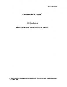
6 To explain this point, we consider modular invariants of extension type. In this case the vacuum of the extended theory is a particular reducible sector of the original theory. It corresponds to an object A in C, but this objects inherits additional structure from the vacuum of the extended theory: The associative OPE induces an associative product on A, which is a morphism m ∈ Hom(A ⊗ A, A). There is also a co-algebra structure, in particular a coproduct ∆ ∈ Hom(A, A ⊗ A). Product and co-product are subject to a number of axioms. Here we highlight just two of them (for the full list see [9]). First, the crossing symmetry between s-channel and t-channel is taken into account by demanding A to be a Frobenius algebra, i.e. to satisfy (idA ⊗ m) ◦ (∆ ⊗ idA ) = ∆ ◦ m = (m ⊗ idA ) ◦ (idA ⊗ ∆) . Pictorially, this is represented as follows:

=

=

Second, the property that A is special includes the relation m ◦ ∆ = idA . Let us give a few examples for symmetric special Frobenius algebras. The relevant algebra for a simple current modular invariant based on a group H of simple currents is M A= J. J∈H

This object admits inequivalent algebra structures which differ by elements in H 2 (H, C× ), corresponding to different choices of discrete torsion. We stress, however, that that our formalism treats simple current modular invariants and exceptional modular invariants on the same footing. For instance, the exceptional invariants of the sl(2) WZW theory of type E6 (at level 10), E7 (level 16) and E8 (level 28) are obtained from the algebras A = 0 ⊕ 6, A = 0 ⊕ 8 ⊕ 16, and A = 0 ⊕ 10 ⊕ 18 ⊕ 28, respectively [12]. The next step in the construction of correlators is to study representations of A. It turns out that A-representations have a direct physical interpretation: they correspond to boundary conditions. A representation theory analogous to the one for vector spaces exists also

7 for algebra objects in the tensor categories that describe Moore-Seiberg data. In particular, there is the notion of an irreducible representation; it corresponds to an elementary boundary condition. For rational CFTs, reducible representations are always fully reducible; they correspond to boundary conditions with non-trivial Chan-Paton multiplicities. Standard tools from representation theory like induced representations or reciprocity theorems, which generalize to tensor categories (see e.g. [12,7]), can be used to work out the list of boundary conditions in many concrete examples and serve as a rigorous justification of the procedure proposed in [6]. We can now finally give a prescription for the Wilson graph in the connecting manifold MX . It beautifully combines the construction of [3,4] with structures familiar [10] from lattice TFTs in two dimensions: ˆ (1) Each bulk insertion point pℓ on X has two preimages pˆ± ℓ on X, which are joined by an interval in MX . We put a Wilson line along each such interval. The image of X in MX intersects this interval in a unique point, which we identify with pℓ ∈ X. (2) Each component of the boundary of X gives rise to a line of fixed points of MX under the Z2 -action. We place a circular Wilson line along each such line of fixed points. ˆ (3) Boundary insertion points qℓ on X have a unique preimage qˆℓ on X. We join qˆℓ by a short Wilson line to the image of qℓ in MX , which results in a trivalent vertex on the relevant circular Wilson line. (4) We place a Wilson line along every edge of an (arbitrarily chosen) triangulation of the image of X in MX . For each bulk insertion we join the perpendicular Wilson line in pℓ by an additional line to an interior point of an arbitrary edge of the face to which pℓ belongs. Similarly one joins the triangulation to every segment of the circular boundary lines. This is the geometric part of the prescription. In addition we must decorate all Wilson lines with labels specifying the corresponding object of the category and choose couplings (morphisms) for the vertices. Our construction is inspired by the situation in two-dimensional lattice TFTs and contains that case as a special example. Here we merely sketch the idea; for more details see [9]: (5) The triangulation and the short Wilson lines that connect the bulk insertion points pℓ to the triangulation are labelled by the object A. (6) To vertices that join three A-lines we assign morphisms that are constructed from the product m on A and from an isomorphism between A and its dual A∨ . (7) To characterize the bulk field inserted at pℓ , we must specify two irreducible objects jℓ± ; they label the Wilson lines that start from the

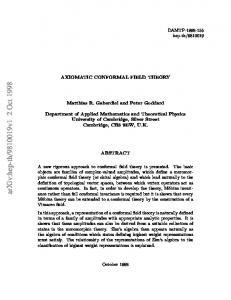
8 ˆ points pˆ± ℓ on X. To account for the coupling to the short A-lines, we need as a third datum for a bulk field a morphism in Hom(A ⊗ jℓ+ , jℓ−∨ ). (Physical bulk fields correspond only to a subspace of these couplings. Couplings in a complement of this subspace completely decouple in all amplitudes.) (8) Each segment of the circular Wilson line corresponds to a boundary condition; it is to be labelled by an A-representation M . Wilson lines of the triangulation that end on such a boundary segment result in a trivalent vertex, to which we assign the representation morphism for M . (9) The boundary fields have a single chiral label kℓ , which labels the short Wilson line from qˆℓ to qℓ . The trivalent vertex that is formed by this Wilson line and the two adjacent boundary conditions M, N requires the choice of a coupling in (a subspace of) Hom(M ⊗kℓ , N ). When X is the disk with three bulk j2−∨ and three boundary insertions, the picture then looks as follows: j1−∨ j3−∨ k3

M2

M3 k1

k2

M1 j1+

j3+ j2+

5.

Results

We have presented a complete and fully general prescription for all correlators on (orientable) world sheets of any topology. One can now prove that this ansatz fulfils two types of consistency conditions: modˆ σ) of arc ular invariance and factorization. First, the group Aut(X, ˆ preserving homeomorphisms of X of degree 1 that commute with the action of σ – the ‘relative modular group’ [2] – acts genuinely on the ˆ of conformal blocks. The correlators on X ˆ can be shown space H(X) to be invariant under this action. This general result contains modular invariance of the torus partition function as a special case. Second, we have compatibility with factorization: By gluing together two insertion points of a world sheet X (either both of them in the bulk or both on the boundary) one gets a world sheet X ′ of different topology. We find that the correlators on X and on X ′ are correctly related by gluing maps.

9 As special cases, our prescription for the correlators allows to compute explicitly partition functions and operator products. Besides being modular invariant, the partition function obtained for the torus without insertions can be shown to possess the usual integrality properties. Similarly, the annulus without insertions yields a representation of the fusion rules by matrices with non-negative integral entries, a so-called NIM-rep. The one-point functions for bulk fields on the disc give the boundary states. Their coefficients can be shown to furnish a classifying algebra [5]. In the simple current case one recovers the boundary states proposed in [8]. Finally, bulk and boundary OPEs can be computed. For modular invariants of extension type, the category CA of A-representations has additional structure. In particular CA is itself a tensor category, and it possesses a ‘good’ duality. In this situation, the annulus coefficients coincide with the fusion rules of CA , the 6j-symbols of CA give the boundary OPE, and the quantum dimension of an object in CA provides the boundary entropy [1] of the corresponding boundary condition. The algebra object A is itself an A-representation and hence corresponds to an (elementary) boundary condition. The algebra of open string states for this boundary condition (in string speak: the quantized algebra of functions on the corresponding brane) gives rise to the category theoretic algebra A ⊗A A ∼ = A. We can therefore conclude: The complete CFT can be reconstructed from the underlying chiral CFT by using only the knowledge of the algebra of open string states for a single boundary condition. This immediately raises the question whether such a reconstruction is also possible from the algebra of open string states of any elementary boundary condition. This is indeed the case: Every elementary boundary condition gives rise to an algebra object from which the same full CFT can be constructed. Therefore the algebra A should not be thought of as an observable quantity – a fact already familiar from lattice topological field theories in two dimensions [10]. The algebras A1 and A2 corresponding to different boundary conditions are, however, closely related: they are Morita equivalent. This means that there exist ˜A (the first a left module of the algebra A1 bimodules A1MA2 and A2M 1 and a right module of A2 , and the second a left module of A2 and a right module of A1 ) such that A1MA2

˜A ) = A1 ⊗A2 (A2M 1

and

˜A ) ⊗A (A MA ) = A2 . (A2M 1 1 2 1

Together with orbifold techniques, Morita equivalence also allows for a deeper understanding of T-duality.

10

6.

Conclusions

Full rational conformal field theories that are based on the chiral data encoded in a modular tensor category C can be obtained from (Morita equivalence classes of) symmetric special Frobenius algebras A in C. We gave a general prescription for the construction of correlation functions on orientable surfaces, including surfaces with boundary. Boundary conditions are in one-to-one correspondence to representations of A. These results allow us to formulate two well-defined classification problems: the one of classifying all full CFTs based on a given chiral CFT, and the one of classifying all boundary conditions that preserve a certain subsymmetry of a given CFT, in the extreme case only conformal symmetry. Except for the Virasoro minimal models, the latter situation is non-rational. We are confident that the structures presented above are flexible enough to be generalized to the non-rational case. In this regard, we expect an intimate relation between the problem of deforming Frobenius algebras in tensor categories and the problem of deforming conformal field theories. Our results should also be extended to include the case of unorientable surfaces, which appear naturally in type I string theories.

Acknowledgments C.S. thanks the organizers of the NATO Advanced Research Workshop on Statistical Field Theories for a stimulating meeting and for the invitation to present this work. Some of the results have been obtained in collaboration with Giovanni Felder and J¨ urg Fr¨ ohlich. We would like to thank them for discussions and for a very pleasant collaboration.

References [1] I. Affleck and A.W.W. Ludwig, Phys. Rev. Lett. 67, 161 (1991) [2] M. Bianchi and A. Sagnotti, Phys. Lett. B 231, 389 (1989) [3] G. Felder, J. Fr¨ ohlich, J. Fuchs, and C. Schweigert, Phys. Rev. Lett. 84, 1659 (2000) [4] G. Felder, J. Fr¨ ohlich, J. Fuchs, and C. Schweigert, preprint ETH-TH/99-30 & PAR-LPTHE 99-45, Compos. Math., in press [5] J. Fuchs and C. Schweigert, Phys. Lett. B 414, 251 (1997) [6] J. Fuchs and C. Schweigert, Phys. Lett. B 490, 163 (2000) [7] J. Fuchs and C. Schweigert, math.CT/0106050, to appear in Fields Inst. Commun. [8] J. Fuchs, L.R. Huiszoon, A.N. Schellekens, C. Schweigert, and J. Walcher, Phys. Lett. B 495, 427 (2000) [9] J. Fuchs, I. Runkel and C. Schweigert, preprint PAR-LPTHE 01-45, hep-th/0110133 [10] M. Fukuma, S. Hosono, and H. Kawai, Commun. Math. Phys. 161, 157 (1994) [11] P. Hoˇrava, J. Geom. and Phys. 21, 1 (1996) [12] A.N. Kirillov and V. Ostrik, preprint math.QA/0101219 [13] V.G. Turaev, Quantum Invariants of Knots and 3-Manifolds (de Gruyter 1994)