Connecting clinical and actuarial prediction with rule-based methods

Please note: This pdf is the accepted author manuscript version of this paper. It may not exactly replicate the final version published in the APA journal. It is not the copy of record. The published version of this paper (of which APA is the copyright holder) can be obtained from Psychological Assessment at www.apa.org/pubs/ journals/pas/.

Connecting clinical and actuarial prediction with rule-based methods Marjolein Fokkema, Niels Smits VU University, Amsterdam

Henk Kelderman

Brenda W.J.H. Penninx

VU University, Amsterdam and Leiden University

Department of Psychiatry and EMGO Institute for Health and Care Research, VU University Medical Center, Amsterdam

Meta-analyses comparing the accuracy of clinical versus actuarial prediction have shown actuarial methods to outperform clinical methods, on average. However, actuarial methods are still not widely used in clinical practice, and there has been a call for the development of actuarial prediction methods for clinical practice. In this paper, we argue that rule-based methods may be more useful than the linear main effect models usually employed in prediction studies, from a data and decision analytic, as well as a practical perspective. In addition, decision rules derived with rule-based methods can be represented as fast and frugal trees, which, unlike main effects models, can be used in a sequential fashion, reducing the number of cues that have to be evaluated before making a prediction. We illustrate the usability of rule-based methods by applying RuleFit, an algorithm for deriving decision rules for classification and regression problems, to a dataset on prediction of the course of depressive and anxiety disorders from Penninx et al. (2011). The RuleFit algorithm provided a model consisting of two simple decision rules, requiring evaluation of only two to four cues. Predictive accuracy of the two-rule model was very similar to that of a logistic regression model incorporating 20 predictor variables, originally applied to the dataset. In addition, the two-rule model required evaluation of only three cues, on average. Therefore, the RuleFit algorithm appears to be a promising method for creating decision tools that are less time consuming and easier to apply in psychological practice, and with accuracy comparable to traditional actuarial methods. Keywords: actuarial prediction, clinical judgment, decision making, linear models, rule-based methods, RuleFit algorithm

Introduction Since publication of Paul Meehl’s “disturbing little book” (Meehl, 1954, 1986), the performance of clinical versus actuarial prediction methods has been a topic of debate and research in psychology (e.g., Ægisd´ottir et al., 2006; Dawes, Faust, & Meehl, 1989; Grove & Meehl, 1996; Grove, Zald, Lebow, Snitz, & Nelson, 2000). In line with Meehl’s (1954) findings, two more recent meta-analyses comparing the accuracy of both prediction methods have shown actuarial prediction to be 10 to 13% more accurate (Ægisd´ottir et al., 2006;

Marjolein Fokkema, Faculty of Psychology and Education, VU University, Amsterdam; Niels Smits, Faculty of Psychology and Education, VU University, Amsterdam; Henk Kelderman, Faculty of Psychology and Education, VU University, Amsterdam, and Faculty of Social Sciences Institute of Psychology, Leiden University; Brenda W.J.H. Penninx, Department of Psychiatry and EMGO Institute for Health and Care Research, VU University Medical Center, Amsterdam. Correspondence concerning this article should be addressed to Marjolein Fokkema, Department of Psychology and Education, Vrije Universiteit Amsterdam, Room 2B73, Van der Boechorststraat 1, 1081BT Amsterdam. Email: [email protected]

Grove et al., 2000), on average. In spite of this evidence, some authors have noted a limited use of actuarial prediction methods in clinical practice (e.g., Kleinmuntz, 1990; Bell & Mellor, 2009). Whereas some have attributed this to the limited value of current actuarial prediction methods for clinical practice (Garb, 1994, 2000), other authors have attributed it to the high demands actuarial methods place on clinicians’ time, information and computational power (Katsikopoulos, Pachur, Machery, & Wallin, 2008; Kleinmuntz, 1990). In any case, there has been a call for the development of new actuarial prediction methods for clinical practice (Garb, 1994, 2000; Spengler, 2012). In this paper, we propose an actuarial prediction method that involves less testing and computation when applied in clinical practice, and with predictive power that may well compete with that of more established actuarial methods based on linear main effects (LME) models. Interestingly, actuarial prediction methods traditionally used are generally restricted to LME models. For example, the majority of studies included in Ægisd´ottir et al. (2006) that provided explicit descriptions of their data-analytic approach, used linear regression, logistic regression or linear discriminant analysis for actuarial prediction prediction. Although LME models may often dominate psychologists’ data-analytic toolbox, they have three drawbacks. First, LME models do not seem to resemble the reasoning pro-

Citation info: Connecting clinical and actuarial prediction with rule-based methods. Fokkema, M., Smits, N., Kelderman, H. and Penninx, B.W.J.H. (in press). Psychological Assessment.

2

MARJOLEIN FOKKEMA, NIELS SMITS

cess of human decision makers in clinical practice. Many authors have found the weighing of cues in human judgment (e.g., Dhami, 2003; Green & Mehr, 1997; Gigerenzer & Goldstein, 1996), and more specifically, judgment by psychologists (e.g, Ganzach, 1995, 1997, 2001; Steadman et al., 2000), to be nonlinear. Psychologists are thus unlikely to make decisions by weighing the values of a large number of variables, like in LME models. Instead, they are likely to use only a small number of cues, and the weights of cues may be dependent on other cue values (e.g., Brannick & Brannick, 1989). Secondly, LME models may provide clinicians with risk factors, but they do not provide direct identification of patients who are at high risk. LME models require calculation of a risk index, by multiplying values of predictor variables by their weights, summing these, and comparing this index to a given cut-off value for deciding whether a patient is at risk. Such calculations are cumbersome to perform, and such models may not conform with clinical reasoning (e.g., Marshall, 1995). In addition, these computations can only be made after all cues are evaluated, although for many patients, evaluation of only a subset of cues may suffice to make a decision. Thirdly, from a data-analytic perspective, LME models may not provide the most accurate or informative results (e.g., Breiman, 2001; Hastie, Tibshirani, & Friedman, 2009). For example, assumptions of normality underlying LME models may be violated in many applications, and LME models are unable to capture potential interaction effects between predictor and outcome variables. In the current paper, we aim to introduce rule-based methods as a tool for actuarial prediction in clinical practice, that does not suffer from the drawbacks described above. The results of rule-based methods may show closer resemblance to the reasoning of psychologists working in applied settings, and allow for direct identification of high- and/or low-risk patients. Due to their interpretability and flexibility, rulebased methods have already gained popularity in the areas of machine learning and data mining (F¨urnkranz, Gamberger, & Lavraˇc, 2012). Furthermore, the decision rules resulting from the application of rule-based methods can be represented as fast and frugal trees (FFTs; Martignon, Vitouch, Takezawa, & Forster, 2003): graphically represented decision tools, developed within the area of heuristical decision making (Gigerenzer & Goldstein, 1996; Gigerenzer, Todd, & the ABC Research Group, 1999). Therefore, we believe rulebased methods may be a promising tool for the application of actuarial prediction in clinical practice. In what follows, we will describe FFTs and rule-based learning algorithms. In the Illustration section, we describe the application of RuleFit (Friedman & Popescu, 2008), a rule-based learning algorithm, to a clinical prediction problem. With RuleFit, we derive simple rules for prediction of the course of depressive and anxiety disorders, using a dataset from the Netherlands Study of Depression and Anxiety (Penninx et al., 2011). To assess the performance of the rule-based model, we will compare its efficiency and accuracy to that of an LME-based prediction model, originally applied to the data. In the Discussion, we describe the advantages and disadvantages of a rule-based approach to clinical

prediction problems.

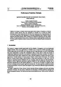
Fast and frugal trees Katsikopoulos et al. (2008) suggested fast and frugal heuristics as a means to ‘bridge the clinical-actuarial divide’. Fast and frugal heuristics (Gigerenzer & Goldstein, 1996) are simple, nonlinear decision rules, which evaluate only a small number of binary input variables, or cues. One of those heuristics is the fast and frugal tree (FFT): a decision tree that evaluates a limited number of cues in a very straightforward manner. By definition, an FFT that evaluates m cues has m + 1 exit nodes, with one exit node for each of the first m − 1 cues and two exit nodes for the last cue (Martignon, Katsikopoulos, & Woike, 2008; Martignon et al., 2003). For example, suppose we want to use the two anxiety items of the five-item Mental Health Inventory (MHI) to assess whether a respondent is at risk for having an anxiety disorder (Cuijpers, Smits, Donker, Ten Have, & de Graaf, 2009; Ware & Sherbourne, 1992). In Figure 1, a (fictitious) FFT for deciding whether a respondent is at risk, using the MHI anxiety items, is depicted. This FFT evaluates two cues, and has three exit nodes. When the answer to the first question or cue (”In the last month, did you feel calm and peaceful?”) is ”yes”, we may immediately decide that this respondent is not at risk for anxiety disorder (Figure 1). However, when the answer is ”no”, interviewing may be continued by presenting the second question or cue to the respondent (”In the last month, did you consider yourself to be a very nervous person?”). If the answer is ”no”, we may decide this respondent is not at risk. In a similar vein, when the answer is ”yes”, we may decide that this patient is at risk for anxiety disorder (Figure 1). FFTs offer several advantages as decision making tools: They require evaluation of only a limited number of cues. In many instances, not every cue in the FFT has to be evaluated, because an exit node is reached early in the tree. Although FFTs require less information for prediction of new classes, their accuracy has been shown to be only slightly lower than that of more complex models based on the same dataset (Jenny, Pachur, Williams, Becker, & Margraf, 2013; Martignon et al., 2008; Smith & Gilhooly, 2006). Finally, the graphical representation of FFTs allows for fast and straightforward application in practical decision making. Current algorithms for creating FFTs 1 , however, have some limitations as well. First, although the graphical tree structure of FFTs appears to convey interaction effects, the algorithms described in Martignon et al. (2003) only optimize overall diagnostic accuracy. The algorithms order cues based on overall sensitivity or specificity of cues, while potential interactions between cues are not taken into account. Secondly, the algorithms do not provide a method for variable selection: cues to be included in the FFT are selected by the user, prior to application of the algorithms. Third, 1 In the remainder of this article, we will distinguish between the algorithms to derive FTTs and graphical representations of FFTs. The term FFT will be used to denote the graphical tree representation, whereas algorithms to derive FFTs will be explicitly denoted as such.

3

CONNECTING CLINICAL AND ACTUARIAL PREDICTION WITH RULE-BASED METHODS

the current algorithms can only deal with dichotomous cues, while in many prediction problems, input variables may be ordinal or continuous.

Classification and regression trees In contrast to the current FFT algorithms, the classification and regression tree (CART) algorithm of Breiman, Friedman, Olshen, and Stone (1984) is able to deal with large numbers of input variables, with categorical, ordinal and continuous in- and output variables, and is able to capture interaction effects as well. The CART algorithm create a decision tree, by partitioning observations into increasingly smaller subgroups, whose members are increasingly similar with respect to an outcome variable. Partitions, or splits, are made using one input variable at a time: in every node, the algorithm selects the variable and splitting point that separate the observations into two subsets for which the distributions of the outcome variable are most different. The result is a decision tree, consisting of branches and nodes. This tree can be used for prediction, by ’dropping’ new observations down the tree (Breiman et al., 1984). For a more extensive description of the CART algorithm, see Berk (2006) or Strobl, Malley, and Tutz (2009). Gigerenzer and Goldstein (1996) and Gigerenzer et al. (1999) have suggested CART as a powerful algorithm for the creation of simple decision making tools, because CART trees, like FFTs evaluate one cue at a time in order to arrive at a final decision. However, the ease with which a decision tree can be communicated or interpreted, diminishes with the number of nodes and branches within a tree (Elomaa, 1994; Quinlan, 1987b). For example, the tree in Figure 1 is easy to comprehend, as it consists of only one branch, and evaluates only two cues. However, a decision tree consisting of many branches, six for example, would be much more difficult to comprehend or communicate. Therefore, CART trees may need to be simplified to improve their usability and communicability.

Rule-based methods One way to simplify decision trees is to convert their branches to decision rules, which are easier to communicate and use (Elomaa, 1994; Quinlan, 1987a, 1987b). Decision rules are statements of the form if [condition], then [decision] (Dembczy´nski, Kotłowski, & Słowi´nski, 2010). Similarly, decision rules used for prediction can be formulated as if [condition], then [prediction]. The condition specifies a set of values of input variables, and the prediction specifies the expected value of the output variable, when an observation satisfies the specified condition. These rules are conjunctive: every one of the arguments has to be met, and if any single condition is not met by an observation, the rule does not apply to the observation. Prediction rules can be represented as an FFT, and vice versa. For example, the FFT in Figure 1 represents the prediction rule: If Q1=‘no’ & Q2=‘yes’, then ‘At risk’. Several algorithms for rule induction have been developed, with the large majority aimed at (binary) classification (e.g., Cohen

& Singer, 1999; Dembczy´nski et al., 2010; Frank & Witten, 1998; Indurkhya & Weiss, 2001; Quinlan, 1993). The RuleFit algorithm of Friedman and Popescu (2008) can deal with both classification and regression problems, and is therefore preeminently suited for prediction problems in clinical psychology, as these may involve categorial as well as continuous outcome variables.

RuleFit algorithm RuleFit is a so-called ensemble method (e.g., Berk, 2006): it combines the predictions of multiple simple prediction functions to make a final prediction. The RuleFit model, as most learning ensembles, takes the form F(x) = a0 +

M X

am fm (x)

(1)

m=1

where F(x) is the linear predictor in a generalized linear model, M is the size of the ensemble, and fm (x) denotes ensemble member m. Ensemble members can be any function of the input variables x; in the case of RuleFit the functions are decision rules. The predictions of the ensemble are a linear combination of the predictions of the ensemble members, with a0 , ..., a M representing weight coefficients. RuleFit derives an ensemble of prediction rules in two stages: first, it generates a large initial ensemble of decision rules fm (x), and second, it estimates the weight coefficients a0 , ..., a M for the final ensemble. Stage one: rule generation. To generate a large initial ensemble of decision rules, RuleFit draws a large number of subsamples of predetermined size of the training dataset, and grows a CART tree on each of the subsamples. Larger subsample size results in more similar subsamples, more similar CART trees, and more similar decision rules. The size of every CART trees grown is determined by a random draw from an exponential distribution, of which the mean is determined by the user. The minimum tree size is two; setting the average tree size to values > 2 allows for the detection of interaction effects. The learning rate of the ensemble can be controlled by setting a shrinkage parameter. This parameter determines the weight given to previously induced ensemble members, when learning new ensemble members. Instead of fitting a tree directly to the data in the current subsample, the tree is fitted to the residual of the predictions of previously induced trees, weighted by the shrinkage parameter. Setting the weight parameter to 0 minimizes the influence of previously induced ensemble members, and results in the tree being fit directly to the data in the current subsample. Setting the weight parameter to 1 maximizes the influence of previously induced ensemble members, and resembles boosting (e.g., Schapire, 2003). Friedman and Popescu (2003) found a shrinkage parameter value of 0.01 to provide the best results. After growing a CART tree, every node of the tree is included as a decision rule in the initial ensemble. To illustrate,

4

MARJOLEIN FOKKEMA, NIELS SMITS

an example of a decision tree from Fokkema, Smits, Kelderman, Carlier, and van Hemert (2014) is presented in Figure 2. Figure 2 represents a classification tree for predicting major depressive disorder diagnoses using total scores on four subscales of a mood and anxiety symptoms questionnaire: AD, GDD, GDA and GDM. The tree has a total of fifteen nodes, and therefore provides fifteen decision rules. For example, node number 10 in Figure 2 can be represented as the rule r10 (x) = I(AD > 76) · I(AD ≤ 81) · I(GDM ≤ 44), where I is an identity function, taking a value of 0 when the condition is not met, and taking a value of 1 when the condition is met. Similarly, node number three can be represented as the rule r3 (x) = I(AD ≤ 76) · I(GDD ≤ 25). Rules rm (x) take a value of 1 when all the conditions of the rule are met, and a value of 0 when any of the conditions of the rule is not met. Stage two: weight estimation. To improve interpretability and counter overfitting, RuleFit creates a final ensemble of prediction functions by a applying a sparse regression of the output variable on the decision rules, in the second stage. Compared to ordinary least squares (OLS), sparse regression methods shrink the coefficients of predictors variables to values closer or equal to zero. This offers two major advantages: lower expected prediction error, due to lower variance of the coefficient estimates, and better interpretability, due to the smaller number of predictors with non-zero coefficients (Hastie et al., 2009). One of four sparse regression methods can be used: ridge, elastic net, lasso, or forward stagewise regression. Each proves a different level of sparsity of the final ensemble (e.g., Zou & Hastie, 2005; Hastie, Taylor, Tibshirani, & Walther, 2007; Tibshirani, 1996). Ridge regression generally shrinks coefficients to smaller, more similar, but nonzero values, compared to the OLS solution. Lasso regression generally shrinks coefficients to smaller values than the OLS solution; it may also shrink coefficient estimates to zero, therefore providing sparser models than with ridge regression. Elastic net regression provides a hybrid of ridge and lasso regression. The forward stagewise regression algorithm initializes by setting coefficients am of all prediction functions fm (x) to zero. Then, the coefficient of the prediction function most strongly correlated with the outcome variable is increased (or decreased, depending on the sign of the correlation) in very small steps (e.g., 0.01). The coefficient of the prediction function is increased (or decreased) in this way, until another prediction function has an equally strong, or stronger correlation with the current residual. Then, the coefficient of that prediction function is increased (or decreased), until another prediction function has an equally strong or stronger correlation with the current residual. This process continues until no predictor has any correlation with the residual anymore. Forward stagewise regression is preferable in case of large numbers of correlated predictors, and yields very sparse models (Hastie et al., 2007), thus improving interpretability. In short, RuleFit creates a large initial ensemble of prediction rules in the first stage, and selects only those rules that improve predictive accuracy in the second stage. This provides the user with a relatively small rule ensemble, that

can be easily interpreted and applied.

Illustration To illustrate the use of the RuleFit algorithm, we apply it to a dataset that was used by Penninx et al. (2011) to find predictors of the course of depressive and anxiety disorders. Penninx et al. (2011) used logistic regression analysis to find sociodemographic and clinical characteristics that predicted psychiatric status (i.e., presence of a depressive or anxiety disorder) after two years. Prediction of the course of these disorders is important, as it offers support for individualized care approaches, in which intensive treatment strategies are reserved for patients at high risk for a chronic course of the disorder. It should be noted that baseline sociodemographic and clinical characteristics can be expected to only partially explain two-year psychiatric status, because other (e.g., environmental, genetic, neurobiological and personality) characteristics also exert influence on the course of depressive and anxiety disorders. Sociodemographic and clinical information, however, is readily available to clinicians, and therefore provides a good starting point for course prediction. Additionally, definitions of chronicity require a two-year time period (Scott, 1988), although predictions over a two-year time period may be expected to be of lower accuracy than predictions over smaller time periods. Any model for the prediction of two-year psychiatric status can therefore be expected to have somewhat limited predictive accuracy, but may nevertheless offer valuable decision-making tools for the allocation of limited health care resources.

Sample Penninx et al. (2011) identified predictors of the course of depressive and anxiety disorders using data from the Netherlands Study of Depression and Anxiety (NESDA; Penninx et al., 2008). This longitudinal study includes 2981 respondents, aged 18 through 65 years. Penninx et al. (2011) used baseline characteristics of respondents with depressive and/or anxiety disorder, to predict psychiatric status (i.e., presence of depressive and/or anxiety disorder) after two years. Therefore, analyses were performed on data from respondents who had a current depressive and/or anxiety disorder at baseline and participated in the follow-up after two years (N=1209). In this sample, mean age was 42.1 years and 66% was female. The NESDA study protocol was centrally approved by the Medical Ethics Review Board, and all respondents provided written informed consent. Further descriptives about the sample can be obtained from Penninx et al. (2011). The logistic regression analysis of Penninx et al. (2011) included 20 predictor variables, consisting of sociodemographic variables, psychiatric indicators and treatment indicators. Penninx et al. (2011) found comorbidity of depressive and anxiety disorders, age, agoraphobia, symptom duration, severity of depressive symptoms, severity of anxiety symptoms and age at disorder onset to be significant predictors

CONNECTING CLINICAL AND ACTUARIAL PREDICTION WITH RULE-BASED METHODS

of psychiatric status after two years. The area under the receiver operating characteristic curve (AUC) for the logistic regression model incorporating all predictor variables, using the same data for estimation and evaluation of the model, was .72 (Penninx et al., 2011).

Outcome and predictor variables Below, we provide a brief description of the variables relevant for prediction of two-year psychiatric status. More detailed descriptions of the variables can be obtained from Penninx et al. (2011). The outcome variable, psychiatric status after two years, was based on the presence of a DSM-IV depressive and/or anxiety disorder at two year follow up (within a six months recency period), as assessed by the Composite International Diagnostic Interview (CIDI, version 2.1; World Health Organization, 1997). Baseline psychiatric status was assessed by means of the baseline CIDI interview, and distinguished between three mutually exclusive categories: pure depression, pure anxiety, and comorbid depression and anxiety. Type of depressive disorder was assessed by means of the baseline CIDI interview as well, and distinguished between three mutually exclusive categories: first episode major depressive disorder (MDD), recurrent MDD, dysthymia. Type of anxiety disorder was assessed by means of the baseline CIDI interview, and distinguished between panic disorder, social phobia, generalized anxiety disorder, and agoraphobia without panic disorder. Age of onset of the index disorder was assessed by means of the baseline CIDI. Duration of depressive and anxiety symptoms was assessed by means of the baseline Life Chart Interview (LCI; Lyketsos, Nestadt, Cwi, Heithoff, & Eaton, 1994). LCI anxiety and depression scores represent the percentage of time in which symptoms of anxiety or depressive disorder were present, during four years before baseline. As the LCI provides separate indicators for anxiety and depression symptoms, the maximum value of both indicators was taken for every respondent. Severity of depressive symptoms was assessed by means of the 30-item Inventory of Depressive Symptomatology (IDS; Rush, Gullion, Basco, Jarrett, & Trivedi, 1996). Severity of anxiety symptoms was assessed by means of the 15-item Fear Questionnaire (FQ; Marks & Mathews, 1979) and the 21-item Beck Anxiety Inventory (BAI; Beck, Epstein, Brown, & Steer, 1988). Sociodemographic characteristics (age, gender, education in years) were obtained with self-report questions.

Analytic models and software To replicate the study by Penninx et al. (2011), and to provide a benchmark based on an LME model, for evaluating the accuracy and efficiency of rule based prediction of psychiatric status in two years, we performed logistic regression (LR) analysis in R (R Development Core Team, 2010). In LR analysis, observations with missing values are deleted (listwise deletion); therefore, we created five imputed datasets using the mi package (Su, Yajima, Gelman, & Hill, 2011)

5

in R, and LR results were pooled across the five imputed datasets. To identify decision rules for predicting psychiatric status after two years, we used the R implementation of the RuleFit algorithm (Friedman & Popescu, 2012), which can be freely downloaded from http://statweb.stanford.edu/˜jhf/R-RuleFit.html. The RuleFit algorithm handles missing data by using all values that are non-missing, so multiple imputation was not necessary for the rule ensemble. RuleFit has a number of settings which can be used to control the complexity of the final ensemble Friedman and Popescu (2008, 2012). In the current study, we have used the default settings of the program, with two exceptions: the model type was set to generate rules only (no linear functions), and forward stagewise regression was selected for creating the final ensemble.

Evaluation of performance Predictive accuracy of the rule ensemble and the logistic regression model was assessed by calculating the area under the curve (AUC). The AUC represents the area under the receiver operating characteristic (ROC) curve for a given model. The ROC curve plots the true positive rate against the false positive rate, for several cutoff values of the class probabilities derived from a given model. AUC values reflect the probability that a randomly chosen observation from the positive class, has a higher model-derived probability of belonging to that class, than a randomly selected observation from the negative class (e.g., Kraemer & Kupfer, 2006). An AUC of 1.0 represents perfect classification accuracy, whereas an AUC of 0.5 represents classification accuracy equal to random guessing. In addition, correct classification rates, sensitivities and specificities were calculated for the LR model and the rule ensemble. The correct classification rate represents the proportion of cases correctly classified. Sensitivity represents the correct classification rate among positively labeled cases, and specificity represents the correct classification rate among negatively labeled cases. Correct classification rate, sensitivity and specificity for a given model may vary, according to the threshold of the model-derived probabilities selected for classifying cases as positive or negative. Thresholds were selected so as to provide equal sensitivity for both models, allowing for straightforward comparison in terms of specificity and correct classification rate. The sensitivity was selected to be the value that maximized the sum of the weighted sensitivity and specificity in the RuleFit model. All measures of predictive accuracy were estimated by means of ten-fold cross validation (CV). Ten-fold CV provides a more accurate and less optimistic estimate of performance of a predictive model, than evaluation of performance with the same data that was used for estimation of the model (Hastie et al., 2009). With ten-fold CV, the original dataset is split into ten random, equally-sized subsets, or folds. For each fold k, the model is retrained, using the observations in the other nine folds. Then, the prediction error is evaluated

6

MARJOLEIN FOKKEMA, NIELS SMITS

using the observations in fold k. This process is repeated for every fold, and the estimated prediction error is averaged over the ten folds. This procedure yields a more realistic estimate of future prediction error of a model, because it does not use the same data for building the model and estimating predictive accuracy. Note that the final model is built using the complete dataset. To evaluate the efficiency of the RuleFit ensemble, we calculated the number of cues that required evaluation to arrive at a final decision for every respondent in the dataset.

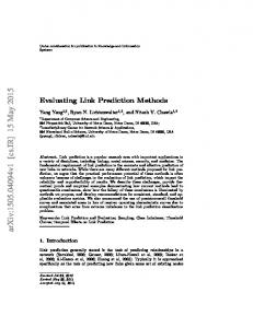
RuleFit ensemble for prediction of two-year psychiatric status Of the 1209 respondents in the dataset, 61.5% had a depressive and/or anxiety disorder at two-year follow up. Consequently, for patients with a current depressive or anxiety disorder, the a-priori odds of having the same psychiatric status two years later were 1.60. The RuleFit ensemble, with rules selected by forward stagewise regression, comprised only two prediction rules. The first rule of the ensemble applied to respondents with an IDS score > 13.50, and anxiety and depressive symptoms for at least 35.9% of the time, over the past four years. This rule had a coefficient of 1.330, representing the estimated increase in the log odds for having the same psychiatric status after two years, when the rule applies. The coefficient indicates that respondents meeting the conditions of this rule have an increased risk of having the same psychiatric status in two years: their odds increase by factor e1.330 = 3.78. Therefore, we formulated it as the following prediction rule: if [IDS score > 13.50 & symptom duration > 35.9%], then [high risk]. This rule is represented as an FFT in the upper panel of Figure 3. The second rule applied to respondents with a BAI score < 9.50, and no comorbid disorder. The second rule had a coefficient of -0.843, the sign indicating that respondents meeting the conditions of this rule have a lowered risk of having the same psychiatric status in two years. For those respondents, the odds of having a depressive or anxiety disorder after two years decrease; they are multiplied by e−0.843 = 0.43. The second prediction rule was formulated as if [BAI score < 9.50 & no comorbid disorder], then [low risk], and is represented as an FFT in the lower panel of Figure 3. Note that a health care worker interested in identifying those who have a high risk of chronicity may only be interested in the first rule. Table 1 presents distributions and estimated probabilities for the two prediction rules. The first rule applied to 24.4% of respondents (Table 1). Patients matching the conditions of this rule, and not the conditions of the second rule, have a high risk of having the same psychiatric status in two years time, with estimated odds of 6.57. The second rule applied to 38.0% of respondents (Table 1). Respondents meeting the conditions of this rule, and not the conditions of the first rule, have a low risk of having the same psychiatric status in two years time, with estimated odds of 0.75. For respondents who did not meet the conditions of either rule (40.8% of respondents; Table 1), the estimated odds

were 1.74, which is slightly higher than the a-priori odds of having the same psychiatric status in two years time. A small proportion (3.2%; Table 1) of respondents met the conditions of the high risk, as well as the low risk rule. For those respondents meeting the conditions of both rules, the estimated odds were 2.83, indicating that they have an elevated risk of having the same psychiatric status in two years time. Therefore, for the 24.4% of patients meeting the conditions of the high risk rule, it may not be necessary to evaluate further cues whether they meet the conditions of the low risk rule, as they have at least an elevated risk of having the same psychiatric status after two years.

Efficiency of RuleFit ensemble The two rules in the RuleFit ensemble required evaluation of at most four cues. For most respondents, however, cue evaluation can be halted earlier. In the sample of 1209 respondents, the median total number of evaluated cues was 3, and the mean was 2.99 cues (SD = 0.545). Halting cue evaluation after the first rule, for respondents who met the criteria of the first rule, would result in a further reduction in the average number of cues to be evaluated, from 2.99 to 2.67.

Predictive performance of RuleFit ensemble and comparison with LR The full logistic regression model incorporated 20 predictor variables, of which five were significant predictors of two year psychiatric status (i.e., had p-values < .05). These were age, IDS score, duration of anxiety and depressive symptoms according to the LCI, age of onset of the index disorder, and BAI score. The AUC for the full model including all 20 predictor variables, as assessed by ten-fold CV, was .689 (Table 2). The accuracy of the RuleFit model was similar to that of the LR model. Based on ten-fold CV, the AUC for the RuleFit model was .686 (Table 2). With sensitivity set equal to .782 for both models, the RuleFit ensemble provided specificity of .447, which was slightly lower than the specificity of .463 for the LR model. Correct classification rates were very similar between the RuleFit ensemble and the LR model: .653 and .659, respectively (Table 2).

Summary The RuleFit algorithm, using forward stagewise regression for selecting the final ensemble, produced two simple decision rules for prediction of psychiatric status of respondents with a current depressive or anxiety disorder. Although the course of psychiatric disorders is determined by many other than sociodemographic and clinical characteristics, these two rules provide a good starting point for course prediction in clinical practice. While the RuleFit ensemble required evaluation of only three cues, on average, to make a prediction, its accuracy was very similar to that of a logistic regression model comprising 20 predictor variables.

CONNECTING CLINICAL AND ACTUARIAL PREDICTION WITH RULE-BASED METHODS

Discussion In the Illustration, we showed that the RuleFit algorithm can provide simple rule ensembles, which may prove highly usable for psychologists working in applied settings. We found the predictive accuracy of rule ensembles to be competitive with that of an LME model which would usually be applied for actuarial prediction. Unlike LME models, rule ensembles are able to convey interaction effects. This not only allows for a more flexible representation of the relationship between predictor variables and the outcome; it also produces results which are more efficient in decision making. Whereas logistic regression models require the values of all (significant) predictor variables to be taken into account for making a prediction, decision rules require evaluation of only a limited number of cues. This is reminiscent of sequential testing, introduced by Cronbach and Gleser (1965), where the aim is to collect new information at every stage of testing; attributes that are redundant given previous outcomes, are neglected. In clinical diagnosis, sequential testing may provide substantial reductions in respondent burden and clinicians’ time needed for making a decision. For example, Fokkema et al. (2014) have shown that sequential testing in clinical diagnosis may provide assessment length reduction of about 50%. In the current study, we found that the number of cues to be evaluated could be reduced by 25 to 33%. The tree-based representation offers an additional improvement in the practical applicability of prediction rules. Applicability may be a key factor in advancing the use of actuarial prediction in clinical practice, as well-validated prediction rules may be available, but still rarely used in practice, possibly due to their complexity. For example, for the Outcome Questionnaire-45 Lambert, Hansen, and Finch (2001)), regression rules for predicting which patients will have a poor treatment response have been proven effective in predicting and improving outcomes, but are rarely used in practice (Hannan et al., 2005; Lambert et al., 2003). Although complexity of the rules and computations required for making predictions may be inconsequential when tests are administered by computer, in practice tests may often be administered in paper-and-pencil versions, or computerized administration and scoring routines may be unavailable to practitioners. In the current study, we have used an ensemble method to derive decision rules. The use of ensemble methods is advantageous, because the predictions of ensemble methods are more accurate than any of their constituent members (Dietterich, 2000; Berk, 2006). However, ensembles consisting of many prediction functions may be difficult for humans to use and interpret. For the RuleFit algorithm, the sparsity settings can be used to adjust the complexity of the final ensemble. The current study, in line with Hastie et al. (2007), indicates that the use of forward stagewise regression to select and determine the weights of prediction rules, provides an ensemble of interpretable size. In addition to a small number of prediction rules in the final ensemble, it may be desirable for the decision rules in

7

an ensemble to be noncompensatory (Einhorn, 1970; Martignon et al., 2008). A model is noncompensatory if the effect of more important variables can not be compensated for by variables of lesser importance (see Martignon et al., 2008 for a more precise definition of noncompensatory models). This results in more efficient decision making: whenever the conditions of a rule have been met, checking the conditions of further rules is unnecessary for making a final decision. In the current study, the RuleFit model was noncompensatory: meeting the conditions of the first rule resulted in a higher risk, regardless of whether the conditions of the second rule were met. However, the RuleFit algorithm does not necessarily provide non-compensatory models, and may provide compensatory models in other instances. Some authors have criticized the use of CART based methodologies for deriving decision rules (e.g., Marshall, 1995, 2001). For example, they argue that some of the decision rules derived from CART trees may be redundant. The RuleFit algorithm counters this issue by the use of sparse regression to determine the weights of the rules. However, some objections, like for example the data-driven nature of machine learning methodologies, remain valid. Therefore, in application and interpretation of the results of rule-based methods, as with all data-analytic methods, predictive accuracy of decision rules should not be confused with biological meaning or diagnostic interpretation. In conclusion, the current study has shown rule-based methods to be a promising tool for the development of actuarial prediction methods, that are easily applicable, efficient and accurate for clinical decision making.

References Ægisd´ottir, S., White, M., Spengler, P., Maugherman, A., Anderson, L., Cook, R., . . . Rush, J. (2006). The meta-analysis of clinical judgment project: Fifty-six years of accumulated research on clinical versus statistical prediction. The Counseling Psychologist, 34(3), 341–382. Beck, A., Epstein, N., Brown, G., & Steer, R. (1988). An inventory for measuring clinical anxiety: psychometric properties. Journal of Consulting and Clinical Psychology, 56(6), 893–897. Bell, I., & Mellor, D. (2009). Clinical judgements: Research and practice. Australian Psychologist, 44(2), 112–121. Berk, R. (2006). An introduction to ensemble methods for data analysis. Sociological methods & research, 34(3), 263–295. Brannick, M., & Brannick, J. (1989). Nonlinear and noncompensatory processes in performance evaluation. Organizational Behavior and Human Decision Processes, 44(1), 97–122. Breiman, L. (2001). Statistical modeling: The two cultures (with comments and a rejoinder by the author). Statistical Science, 16(3), 199–231. Breiman, L., Friedman, J., Olshen, R., & Stone, C. (1984). Classification and regression trees. New York: Wadsworth. Cohen, W., & Singer, Y. (1999). A simple, fast, and effective rule learner. In Proceedings of the national conference on artificial intelligence (pp. 335–342). Cronbach, L., & Gleser, G. (1965). Psychological tests and personnel decisions. Urbana, IL: University of Illionois Press. Cuijpers, P., Smits, N., Donker, T., Ten Have, M., & de Graaf, R. (2009). Screening for mood and anxiety disorders with the five-

8

MARJOLEIN FOKKEMA, NIELS SMITS

item, the three-item, and the two-item Mental Health Inventory. Psychiatry Research, 168(3), 250–255. Dawes, R., Faust, D., & Meehl, P. (1989). Clinical versus actuarial judgment. Science, 243(4899), 1668–1674. Dembczy´nski, K., Kotłowski, W., & Słowi´nski, R. (2010). ENDER: a statistical framework for boosting decision rules. Data Mining and Knowledge Discovery, 21(1), 52–90. Dhami, M. (2003). Psychological models of professional decision making. Psychological Science, 14(2), 175–180. Dietterich, T. (2000). Ensemble methods in machine learning. Multiple classifier systems, 1–15. Einhorn, H. (1970). The use of nonlinear, noncompensatory models in decision making. Psychological Bulletin, 73(3), 221–230. Elomaa, T. (1994). Machine Learning: Proceedings of the Eleventh International Conference (New Brunswick, NJ). In W. Cohen & H. Hirsh (Eds.), (pp. 62–69). San Francisco, CA: Morgan Kaufmann. Fokkema, M., Smits, N., Kelderman, H., Carlier, I., & van Hemert, A. (2014). Combining decision trees and stochastic curtailment for assessment length reduction of test batteries used for classification. Applied Psychological Measurement, 38(1), 3–17. Frank, E., & Witten, I. (1998). Generating accurate rule sets without global optimization. In Proceedings of the fifteenth international conference on machine learning (pp. 144–151). Friedman, J., & Popescu, B. (2003). Importance sampled learning ensembles [Technical Report]. Stanford University. (http://www-stat.stanford.edu/ jhf/ftp/isle.pdf) Friedman, J., & Popescu, B. (2008). Predictive learning via rule ensembles. The Annals of Applied Statistics, 916–954. Friedman, J., & Popescu, B. (2012). Rulefit (version 3) [Computer software]. (Available from http://www-stat.stanford.edu/ jhf/RRuleFit.html) F¨urnkranz, J., Gamberger, D., & Lavraˇc, N. (2012). Foundations of rule learning. Berlin Heidelberg: Springer-Verlag. Ganzach, Y. (1995). Nonlinear models of clinical judgment: Meehl’s data revisited. Psychological Bulletin, 118(3), 422– 429. Ganzach, Y. (1997). Theory and configurality in clinical judgments of expert and novice psychologists. Journal of Applied Psychology, 82(6), 954–960. Ganzach, Y. (2001). Nonlinear models of clinical judgment: Communal nonlinearity and nonlinear accuracy. Psychological Science, 12(5), 403–407. Garb, H. (1994). Toward a second generation of statistical prediction rules in psychodiagnosis and personality assessment. Computers in Human Behavior, 10(3), 377–394. Garb, H. (2000). Computers will become increasingly important for psychological assessment: Not that there’s anything wrong with that. Psychological Assessment, 12(1), 31–39. Gigerenzer, G., & Goldstein, D. (1996). Reasoning the fast and frugal way: models of bounded rationality. Psychological Review, 103(4), 650–669. Gigerenzer, G., Todd, P., & the ABC Research Group. (1999). Simple heuristics that make us smart. New York, NY: Oxford University Press. Green, L., & Mehr, D. (1997). What alters physicians’ decisions to admit to the coronary care unit? Journal of Family Practice, 45(3), 219–226. Grove, W., & Meehl, P. (1996). Comparative efficiency of informal (subjective, impressionistic) and formal (mechanical, algorithmic) prediction procedures: The clinical-statistical controversy. Psychology, Public Policy, and Law, 2, 293–635.

Grove, W., Zald, D., Lebow, B., Snitz, B., & Nelson, C. (2000). Clinical versus mechanical prediction: a meta-analysis. Psychological Assessment, 12(1), 19. Hannan, C., Lambert, M., Harmon, C., Nielsen, S., Smart, D., Shimokawa, K., & Sutton, S. (2005). A lab test and algorithms for identifying clients at risk for treatment failure. Journal of Clinical Psychology, 61(2), 155–163. Hastie, T., Taylor, J., Tibshirani, R., & Walther, G. (2007). Forward stagewise regression and the monotone lasso. Electronic Journal of Statistics, 1, 1–29. Hastie, T., Tibshirani, R., & Friedman, J. (2009). The elements of statistical learning (2nd ed.). New York, NJ: Springer. Indurkhya, N., & Weiss, S. (2001). Solving regression problems with rule-based ensemble classifiers. In Proceedings of the seventh ACM SIGKDD International Conference on Knowledge Discovery and Data Mining (pp. 287–292). Jenny, M., Pachur, T., Williams, S., Becker, E., & Margraf, J. (2013). Simple rules for detecting depression. Journal of Applied Research in Memory and Cognition. Retrieved from http://dx.doi.org/10.1016/j.jarmac.2013.06.001 Katsikopoulos, K., Pachur, T., Machery, E., & Wallin, A. (2008). From Meehl to fast and frugal heuristics (and back): New insights into how to bridge the clinical–actuarial divide. Theory & Psychology, 18(4), 443–464. Kleinmuntz, B. (1990). Why we still use our heads instead of formulas: toward an integrative approach. Psychological Bulletin, 107(3), 296–310. Kraemer, H., & Kupfer, D. (2006). Size of treatment effects and their importance to clinical research and practice. Biological Psychiatry, 59(11), 990–996. Lambert, M., Hansen, N., & Finch, A. (2001). Patient-focused research: Using patient outcome data to enhance treatment effects. Journal of Consulting and Clinical Psychology, 69(2), 159. Lambert, M., Whipple, J., Hawkins, E., Vermeersch, D., Nielsen, S., & Smart, D. (2003). Is it time for clinicians to routinely track patient outcome? a meta-analysis. Clinical Psychology: Science and Practice, 10(3), 288–301. Lyketsos, C., Nestadt, G., Cwi, J., Heithoff, K., & Eaton, W. (1994). The Life Chart Interview: a standardized method to describe the course of psychopathology. International Journal of Methods in Psychiatric Research, 4(3), 143–155. Marks, I., & Mathews, A. (1979). Brief standard self-rating for phobic patients. Behaviour Research and Therapy, 17(3), 263– 267. Marshall, R. (1995). A program to implement a search method for identification of clinical subgroups. Statistics in Medicine, 14(24), 2645–2659. Marshall, R. (2001). The use of classification and regression trees in clinical epidemiology. Journal of Clinical Epidemiology, 54(6), 603–609. Martignon, L., Katsikopoulos, K., & Woike, J. (2008). Categorization with limited resources: A family of simple heuristics. Journal of Mathematical Psychology, 52(6), 352–361. Martignon, L., Vitouch, O., Takezawa, M., & Forster, M. (2003). Thinking: Psychological perspective on reasoning, judgment, and decision making. In D. Hardman & L. Macchi (Eds.), (pp. 189–211). West Sussex, England: John Wiley & Sons. Meehl, P. (1954). Clinical vs. statistical prediction: A theoretical analysis and a review of the evidence. Minneapolis: University of Minnesota Press. Meehl, P. (1986). Causes and effects of my disturbing little book. Journal of Personality Assessment, 50(3), 370–375.

CONNECTING CLINICAL AND ACTUARIAL PREDICTION WITH RULE-BASED METHODS

Penninx, B., Beekman, A., Smit, J., Zitman, F., Nolen, W., Spinhoven, P., . . . Van Dyck, R. (2008). The Netherlands Study of Depression and Anxiety (NESDA): rationale, objectives and methods. International Journal of Methods in Psychiatric Research, 17(3), 121–140. Penninx, B., Nolen, W., Lamers, F., Zitman, F., Smit, J., Spinhoven, P., . . . Beekman, A. (2011). Two-year course of depressive and anxiety disorders: Results from the Netherlands Study of Depression and Anxiety (NESDA). Journal of Affective Disorders, 133(1), 76–85. Quinlan, J. (1987a). Generating production rules from decision trees. In Proceedings of the tenth international joint conference on artificial intelligence (Vol. 1, pp. 304–307). Quinlan, J. (1987b). Simplifying decision trees. International Journal of Man-Machine Studies, 27(3), 221–234. Quinlan, J. (1993). C4.5: programs for machine learning. Morgan Kaufmann Publishers. R Development Core Team. (2010). R: A language and environment for statistical computing [Computer software manual]. Vienna, Austria. Retrieved from http://www.R-project.org Rush, A., Gullion, C., Basco, M., Jarrett, R., & Trivedi, M. (1996). The inventory of depressive symptomatology (IDS): psychometric properties. Psychological Medicine, 26(3), 477–486. Schapire, R. (2003). The boosting approach to machine learning: An overview. In Nonlinear estimation and classification (pp. 149–171). Springer. Scott, J. (1988). Chronic depression. The British Journal of Psychiatry, 153(3), 287–297. Smith, L., & Gilhooly, K. (2006). Regression versus fast and frugal

9

models of decision-making: The case of prescribing for depression. Applied Cognitive Psychology, 20(2), 265–274. Spengler, P. (2012). Handbook of psychology: Assessment psychology. In I. Weiner, J. Graham, & J. Naglieri (Eds.), (2nd ed., pp. 26–49). Hoboken, NJ: Wiley. Steadman, H., Silver, E., Monahan, J., Appelbaum, P., Robbins, P., Mulvey, E., . . . Banks, S. (2000). A classification tree approach to the development of actuarial violence risk assessment tools. Law and Human Behavior, 24(1), 83–100. Strobl, C., Malley, J., & Tutz, G. (2009). An introduction to recursive partitioning: Rationale, application, and characteristics of classification and regression trees, bagging, and random forests. Psychological Methods, 14(4), 323–348. Su, Y.-S., Yajima, M., Gelman, A., & Hill, J. (2011). Multiple imputation with diagnostics (mi) in R: Opening windows into the black box. Journal of Statistical Software, 45(2), 1–31. Tibshirani, R. (1996). Regression shrinkage and selection via the Lasso. Journal of the Royal Statistical Society. Series B (Methodological), 267–2f88. Ware, J., & Sherbourne, C. (1992). The MOS Short-Form Health Survey (SF-36): I.Conceptual framework and item selection. Medical Care, 30, 473–483. World Health Organization. (1997). Composite International Diagnostic Interview (CIDI): Version 2.1. Geneva: World Health Organization. Zou, H., & Hastie, T. (2005). Regularization and variable selection via the elastic net. Journal of the Royal Statistical Society: Series B (Statistical Methodology), 67(2), 301–320.

Connecting clinical and actuarial prediction with rule-based methods 31

Table 1 Frequencies and estimated probabilities of high- and low-risk rules.

Low-risk rule

High-risk rule

0

1

Total

0

1

Total

frequency

493 (40.78%)

421 (34.82%)

914 (75.60%)

odds (PP)

1.74 (0.63)

0.75 (0.35)

frequency

256 (21.17%)

39 (3.23%)

odds (PP)

6.57 (0.87)

2.83 (0.74)

frequency

749 (61.95%)

460 (38.05%)

295 (24.40%)

1209 (100%)

Note. A value of 0 for a rule indicates that the rule does not apply; a value of 0 indicates that the rule applies. PP = posterior probability of having the same psychiatric status after two years.

Connecting clinical and actuarial prediction with rule-based methods 32

Table 2 Predictive performance of the logistic regression model with four predictor variables and the RuleFit ensemble, based on ten-fold cross validation.

LR

RuleFit

AUC

0.689

0.686

sensitivity

0.782

0.782

specificity

0.463

0.447

CCR

0.659

0.653

Note. Values for logistic regression were averaged across five imputed data sets. Sensitivities for both methods were set equal to allow for comparison of specificity and correct classification rate. LR = logistic regression; CCR = correct classification rate.

Connecting clinical and actuarial prediction with rule-based methods 33 Figure Captions Figure 1. Example fast and frugal tree for at risk and not at risk anxiety disorder classification. Figure 2. Example decision tree from Fokkema et al. 2014 Figure 3. Two fast and frugal trees for prediction of psychiatric status after two years: high risk (upper panel) and low risk (lower panel)

Q1: In the last month, did you feel calm and peaceful? no

yes

Q2: In the last month, did you consider exit yourself to be a very nervous person? yes

at risk

no

exit

IDS > 13.5? yes

no

symptom duration > 35.9%?

exit

yes

no

high risk

exit

comorbid depression and anxiety? yes

no

BAI > 9.5? no

low risk

exit

yes

exit