vehicle is captured by the Poisson Arrival Location Model. (PALM). The actual .... the route according to a velocity field v(x, t), it can be deterministic or density ...
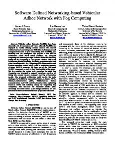
Connectivity Dynamics for Vehicular Ad-hoc Networks in Signalized Road Systems Ivan Wang-Hei Ho*†, Kin K. Leung*, John W. Polak† Department of Electrical and Electronic Engineering, Imperial College London † Centre for Transport Studies, Imperial College London {wh.ho, kin.leung, j.polak}@imperial.ac.uk
*
Abstract – In this paper, we analyze the connectivity dynamics of vehicular ad-hoc networks in a generic signalized urban route. Given the velocity profile of an urban route as a function of space and time, we utilize a fluid model to characterize the general vehicular traffic flow, and a stochastic model to capture the randomness of individual vehicle. From the fluid and stochastic models, we can acquire respectively the densities of the mean number of vehicles along the road and the corresponding distribution. With the knowledge of the vehicular density dynamics, we determine the probability that the communication network is fully connected, i.e., each node can communicate with every other node through a multi-hop path, and the problem is also investigated for a general case of a k-connected network. To closely approximate the practical road conditions, we use a density-dependent velocity profile to approximate vehicle interactions and capture the shockwave propagation at traffic signals. We confirm the accuracy of the connectivity analysis through simulations and show that the analytical results are good approximations even when vehicles interact with each other as their movement is controlled by traffic lights. We also illustrate that system engineering and planning for optimizing connectivity in the communication networks can be carried out with the results in this paper. Index Terms – Vehicular Ad-Hoc Network, Connectivity Dynamics, Stochastic Traffic Model, Signalized Road System, Vehicle Interaction, Transmission Range Adjustment. I. INTRODUCTION In a Vehicular Ad-hoc Network (VANET), vehicles communicate with each other and possibly with road-side infrastructure nodes. Node connectivity and the amount of data that can be exchanged are limited by the duration and quality of the communication links established among nodes, which are determined by the space and time dynamics of moving vehicles. To capture such dynamics in our connectivity analysis, we modify the stochastic traffic model proposed in [1,2] for modeling vehicular traffic in signalized urban road systems. The stochastic traffic model uses a deterministic fluid model to characterize the space and time dynamics of vehicle movements, which is driven by a velocity profile as a function of space and time. In real practice, empirical velocity measurements from GPS devices can serve as an input to the model. The mean density profile, again as a function of space and time, is readily computable from the conservation equations in the fluid model. The randomness of individual vehicle is captured by the Poisson Arrival Location Model (PALM). The actual number of vehicles in a given road
section at a certain time instance has Poisson distribution according to previous PALM results in [1,3] given that the arrival of vehicles follow a non-homogeneous Poisson process and the velocity profile is independent of other parameters such as vehicular density. To closely represent the practical road condition, we attempt to introduce a density-dependent velocity profile to characterize vehicle interactions and shockwave propagation at traffic signals, which has not been considered in previous PALM work [1,2]. But of course, the PALM no longer applies in principle with vehicle interactions due to the existence of dependency. So, we treat the results in the presence of vehicle interactions as approximations, and validate them through simulations in this paper. Through the vehicular density dynamics computed from the stochastic traffic model, we determine the distribution of a node’s location on the urban route, and derive the probability that the entire communication network in the road segment is connected in a multi-hop manner, and the problem is further investigated for a general case of a k-connected network. In essence, we show that the analysis is a valid approximation even when extra randomness is inherited from vehicular interactions and traffic signals. To illustrate the applicability of our results, we demonstrate how the connectivity knowledge can facilitate the adjustment of transmission ranges of vehicles to prevent network disconnection and boost the overall communication connectivity. Related Work There are a number of studies on node connectivity in Mobile Ad-hoc Networks (MANETs). For instance, [4] shows that if the radio transmission range of n nodes that are placed uniformly and independently in a disc of unit area is set to r0 = [(log n + c(n)) / nπ]1/2, the resulting wireless multi-hop network is asymptotically connected with probability one if and only if c(n) Æ ∞. Reference [5] investigates the radio range assignment problem, and obtains bounds for the probability that a node is isolated and the network is connected on a one-dimensional line. On the other hand, [6] examines the node density threshold for achieving full connectivity in both 1-D and 2-D ad-hoc network. [7,8] study the relation between the minimum node degree and k-connectivity in a random graph, and explore the minimum radio transmission range r0 for achieving a fully connected ad-hoc network for a given node density. Most of the existing studies assume that nodes are uniformly random distributed in an area and they are either stationary or move according to the random waypoint model
2 [8], which are obviously inadequate to capture the spatial distribution of vehicles and their movements. In fact, vehicle movements, particularly in urban environments, are restricted by the road topologies, buildings, etc., and affected by traffic density, which is determined by road capacity, traffic control and driver behaviors. There are also recent works that aim to model connectivity of vehicles on a one-dimensional highway. [9] assumes the space headway between vehicles is exponentially distributed, and introduces a robustness factor to capture the effect of disturbance on VANET connectivity. [10] assumes a continuous-time mobility model where movement of each node is a function of time consisting of a sequence of random intervals that is exponential distributed, and during each interval, a node moves at a constant speed which is independently chosen from a normal distribution. Based on this synthetic mobility model, the author derived the mean cluster size and the probability that the nodes will form a single cluster under the assumption that vehicles arrive according to a Poisson process. These previous studies, however, lack of a realistic traffic model to adequately capture node density and its influence on vehicle speed, which are significant in determining connectivity, especially in urban road systems where strong interactions among neighboring vehicles exist. The rest of the paper is organized as follows. Section II provides the background information of the stochastic traffic model (fluid and stochastic models) for computing vehicular density. Section III presents the connectivity analysis with and without the consideration of vehicle interactions. Section IV extends the investigation to the general case of k-connectivity in the network. Section V provides numerical results to verify our analysis. Section VI presents potential applications of the connectivity modeling on transmission range adjustment for boosting overall network connectivity. Finally, Section VII concludes the paper. II. STOCHASTIC TRAFFIC MODEL In this section, we define the system model and provide background information of the fluid and stochastic models, from which we can acquire the vehicular density dynamics in signalized urban routes for VANET connectivity analysis. We consider traffic in a one-way, single-lane, semiinfinite signalized urban road (or route) as shown in Figure 1. Although the road is fed with traffic from adjacent streets, the one-way road under consideration is the one running from the left to the right in the figure. More complicated road topology can be represented by superposing multiple versions of urban routes. Let our location space to be the interval [0, ∞), the boundary point 0 is the spatial origin, and it marks the starting point of the road. The arrival process {A(t) | -∞ < t < ∞} counts the number of arrivals to the first segment of the route up to time t, which we assume is finite with probability 1, and is characterized by a non-negative and integrable external arrival rate function α(t). Furthermore, the route consists of a number of road segments indexed by i = 1, 2, 3,…, and traffic lights are located at the junctions of road segments, where vehicles can leave and join the route. We let the location of the i-th junction (or traffic light) between road segments i and i+1 be xi.
Figure 1. The road configuration considered in this paper.
A. Deterministic Fluid Model The fluid model is a kind of continuum traffic flow models, which reduces laws of traffic to a partial differential equation (PDE) that may be studied as elegantly and simply as other physical phenomena that are also governed by PDE’s. The major difference between our fluid model and other continuum models is that we model vehicle motions with a velocity profile, vehicles at location x and time t move forward the route according to a velocity field v(x, t), it can be deterministic or density dependent. Vehicles stop at road junctions for a red signal, which can be reflected and modeled by the velocity profile. However, continuum model alone is unable to capture traffic instability and the randomness of individual vehicle, therefore, we couple the fluid model with the stochastic model in the next section as a remedy. To begin with, we will describe the fluid dynamic conservation equations and corresponding notations that hold for the general systems. Let N(x, t) be the number of vehicles in location (0, x] at time t, and n(x, t) be the density of vehicles in location (0, x] at time t. Thus, ∂N ( x, t ) (1) . n ( x, t ) = ∂x Let Q(x, t) be the number of vehicles moving past position x before time t. Then the flow rate q(x, t) is defined by ∂Q ( x, t ) . q ( x, t ) = (2) ∂x Let C+(x, t) and C–(x, t) be the number of vehicles arriving to and departing from the route in location (0, x] during time interval (-∞, t], respectively. Then the associated rate densities are respectively
c + ( x, t ) =
2
+
∂ C ( x, t )
c − ( x, t ) =
2
−
∂ C ( x, t )
. (3) ∂x∂t ∂x∂t Assuming all traffic moves only from left to right down the positive real line, then the four variables N, Q, C+, Csatisfy the following conservation relation: and
+
−
C ( x, t ) = N ( x, t ) + Q ( x, t ) + C ( x, t )
(4)
2
By applying the operator ∂ /(∂x∂t ) to (4), we have the partial differential equation ∂n( x, t ) ∂q ( x, t ) + − + = c ( x, t ) − c ( x, t ). (5) ∂t ∂x According to traffic flow theory [11], we have q ( x, t ) = n ( x, t )v ( x, t ). By substituting (6) into (5), we have ∂n( x, t ) ∂ [ n( x, t )v ( x , t ) ] + − + = c ( x, t ) − c ( x, t ). ∂t ∂x
(6)
(7)
3 The resulting partial differential equation (7) is a onedimensional version of the generalized conservation law for fluid motion [12]. This equation governs the mean behavior of any stochastic traffic model. For the ease of solving (7), we introduce an additional assumption to convert the partial differential equation (PDE) to an ordinary differential equation (ODE). Let the location x as a time function, x(t), be given by dx (t ) = v ( x (t ), t ). (8) dt dn ( x (t ), t ) ∂n( x, t ) dx (t ) ∂n( x, t ) = ⋅ + , and by By chain rule, dt dt ∂x ∂t substituting (7) and (8) into this equation, we have dn ( x (t ), t ) dt
+
−
= c ( x (t ), t ) − c ( x (t ), t ) −
∂v ( x, t ) ∂x
n( x (t ), t ). (9)
Due to the partial derivative of v(x, t) w.r.t. x in (9), it is ODE if and only if v(x, t) is not a function of n(x, t). Note that though we introduce the use of a density-dependent velocity profile later on, we still solve the ODE’s for the mean number of vehicles as an approximation in Section V. We assume that vehicles arrive at the first route segment according to an external arrival rate function α(t). If we consider the fleet of vehicles keep moving along the route without vehicles joining or leaving at junctions (e.g., buses move along a bus route). c+(x, t) = α(t)δ(x) and c–(x, t) = 0, where lim
ε →0
x +ε
∫x −ε δ ( y )dy = 1 if x = 0 and 0 otherwise.
+
(10)
i
As for vehicles leaving the route, we use ρi(t) to denote the fraction of vehicles departing when they pass by the i-th junction at time t. If these departing vehicles leave at the same velocity as they move forward along the route, then −
c ( x, t ) = β ( x, t ) n( x, t ) , where
β ( x , t ) = v ( x, t )∑ ρi (t )δ ( x − xi ).
c − ( x, t ) =
−
2
∂ E[C ( x, t )]
. ∂x∂t ∂x∂t The general stochastic model can be of any distributions depending on the arrival process of vehicles, and the equations in the deterministic fluid dynamic model continue to hold regardless the distribution of the stochastic model. In this paper, we specifically consider a Poisson arrival location model (PALM). Again, the fluid dynamic model is not dependent on the Poisson assumption; they hold as long as the arrival process A is an arbitrary point process with timedependent arrival-rate function α. With PALM, the arrival process {A(t) | -∞ < t < ∞} for vehicles to arrive at the first road segment of the route is a non-homogeneous Poisson process with non-negative and integrable external arrival rate function α(t). That is, the number of arrivals in the interval (t1, t2] is Poisson with mean t2
∫t
1
and
α ( s ) ds .
According to [1,3], we can construct N(x, t), the random number of vehicles within the range (0, x] at time t, via stochastic integration starting with the Poisson process A, where A(t) counts the number of vehicles arriving to the road segment up to time t. t
N ( x, t ) =
∫
σ ( x ,t )
A( t )
1{L
s
( t )∈(0, x ]} dA( s ) =
∑ 1{L
n = A (σ ( x ,t ))
Aˆ n
}
( t )∈(0, x ]
(12)
Hence, for all real t, {N(x, t) | x ≥ 0} is a Poisson process with
For the case that there are vehicles join and leave the route at road junctions, let us use ξi(t) to denote the external arrival rate of vehicles at the i-th junction at time t. Then we have
c ( x, t ) = α (t )δ ( x ) + ∑ ξ i (t )δ ( x − xi ).
+
2
∂ E[C ( x, t )]
c + ( x, t ) =
(11)
i
B. Stochastic Model In contrast to the deterministic fluid model, the stochastic model captures the stochastic fluctuations of the quantities of interest. When the two models are coupled with each other to form the stochastic traffic model, the solutions from the PDE’s or ODE’s describe the expected number of vehicles, and the actual number of vehicles is captured by the additional distribution information from the stochastic model. From now on, the densities n(x, t) and q(x, t) are defined as the partial derivatives of expected values, that is, ∂E[N ( x, t )] ∂E[Q ( x, t )] n ( x, t ) = and q ( x, t ) = . ∂x ∂x Similarly, the rate densities c+(x, t) and c-(x, t) are the second partial derivatives of expected values, that is,
E[N ( x, t )] =
t
∫σ
( x ,t )
α ( s ) ds.
(13)
where Aˆ n is the nth jump time of A, counting backward from time t. 1B is an indicator function such that it returns 1 if B is true and 0 otherwise. Ls(t) is the location process, which specifies the position of the vehicle on the road segment at time t that arrived at time s. Let σ(x, t) denote the route entrance time for a vehicle to be in position x at time t. For vehicles that arrive to the route before σ(x, t), it will be past position x by time t. On the other hand, for vehicles arrive after σ(x, t), it will be still in position x at time t. Therefore, as long as we model the traffic flow or even traffic signals through a deterministic velocity field as a function of space and time, and all the vehicles do not interact with each other, the Poisson distributional conclusion in [1,3] remains valid. In Section V, we approximate vehicular interactions through a density-dependent velocity profile. In that case, the stochastic model in principle is invalid, and the Poisson property no longer holds as we cannot determine if a car arrives at time s will have passed location x at time t with the density-dependent velocity profile. However, we found from simulations that the Poisson property and stochastic independence of the model can still be primarily retained when the traffic load is not too high even in the presence of vehicle interactions. Thus, we treat the results with consideration of vehicle interactions as approximations, and confirm their accuracy through simulations. The reader is referred to Section V for details.
4 III. VANET CONNECTIVITY ANALYSIS With the knowledge of the vehicular density dynamics from the stochastic traffic model, we determine in this section the probability that the network within an urban road segment is connected, and extend the investigation to k-connectivity of the network. To model wireless transmission between vehicles, a radio link model is assumed in which each vehicle has a transmission range r, two vehicles are able to communicate (or are connected) directly with each other via a wireless link if the Euclidean distance between them is less than or equal to r. In a one-dimensional ad-hoc network, a node is said to be disconnected from the forward network if it is not connected to any forward neighbors in the network (e.g., node 2 in Figure 2), where ‘forward neighbors’ here represents nodes that are on the right of the considered node assuming that the stream of traffic moves from left to right. A network is said to be connected if for every pair of nodes there exists a path (that is composite of one or more number of communication links) between them, and otherwise it is disconnected. For the connectivity of a one-dimensional network, the following definition holds. Definition 1: For a one-dimensional ad-hoc network, it is connected if and only if there does not exist any nodes in the network that are not connected to any of the forward nodes. In another words, the network is disconnected if the separation between any two adjacent nodes is great than r as illustrated in Figure 2. Therefore, the probability that the network in a road segment is connected is equivalent to the probability that no nodes got isolated from the forward network. The reader is referred to the proof of Proposition 1, which considers the general case of a k-connected network. 0
1
2
d0
d1
3
4
d2 > r
d3
5
d4
A. Connectivity without Vehicle Interactions For analytical simplicity, we cease to focus on time dynamics in this subsection, and assume the system has reached a steady state with respect to time. Thus, all system variables and parameters (including the velocity profile) become independent of time. For this reason, we simply drop the variable t from our previously defined notation. We define N(xa, xb) = N(xb) – N(xa), where xb > xa, as the number of vehicles in the region (xa, xb]. According to the stochastic model, the actual number of vehicles distributed within a road region is Poisson distributed. Thus, we can acquire from it the probability that a specific number of vehicles are located within a road region, which is given by
P ( N ( x) = n ) = P ( N ( xa , xb ) = n ) = where E[ N ( x )] =
∫
x 0
n(u ) du .
n!
n
e
− E [N ( x )]
E[N ( xa , xb )] n!
(14)
n
e
− E [N ( xa , xb )]
d I i (t ) =
(15)
t
∫ t − I v( s)ds
(16)
i
where Ii is the inter-arrival time between the i-th and i+1-st arrivals. We are interested in finding the critical inter-arrival time of the road, Tc, such that if Ii ≤ Tc, the i-th and i+1-st cars will remain connected throughout the whole journey. Or on the other hand, if Ii > Tc, the maximum separation between the two cars in the road segment will be greater than r. We have
{
}
max dTc (t ) = max t∈Ω
t∈Ω
{∫
t t −Tc
}
v ( s ) ds = r
(17)
where Ω is the set of time instances such that the i-th and i+1st cars co-exist in the road segment. Given the velocity profile, we are able to find Tc as a function of r. For Poisson arrival process with parameter α, P(Ii ≤ Tc) = 1 – e–αTc, let it be pc. Therefore, the probability that the entire network remains connected (conditioning on that the population size of the road is non-zero, i.e., N(L) > 0) is 1 ∞ j −1 P (net con) = pc P ( N ( L ) = j ). (18) j =1 1 − P ( N ( L ) = 0) Since the number of cars in the road segment has a Poisson distribution with parameter E[N(L)], which can be computed from the fluid model, by substituting (14) into (18), we have
∑
P (net con) =
Figure 2. Disconnection in a one-dimensional network.
E[N ( x )]
Consider a road segment of length L, cars arrive at location 0 as a homogeneous Poisson process with mean rate α, and assume there are no cars joining and leaving the urban route at junctions. Since we assume the system has reached a steady state with respect to time, the velocity profile is only a function of space but independent of time. Thus, every car that travels through the road segment will have the same velocitytime graph with regard to its arrival time, let us denote it with v(s). At time t, the physical separation between the i-th and the i+1-st cars is
(e
pc E [ N ( L )]
(
pc e
E [ N ( L )]
). − 1)
−1
(19)
B. Connectivity with Vehicle Interactions Subsection A above gives us an exact treatment of modeling the spatial separations between vehicles and connectivity of the network. Strictly speaking, when vehicle interactions are considered, the stochastic model is no longer valid due to the existence of dependency. So, we can only do approximation here and use simulation to evaluate its validity. For velocity profile that is a function of both the space and time, and with vehicle interactions, we approximate the probability of connectivity based on the results of the fluid model, which captures the time and space dynamics as well as vehicular interactions. We now consider a specific time instance t0, and thus the variable t is again simply dropped from our notation. The probability over a period of time can be obtained by taking the time-average of multiple time instances. Again, we consider a road segment with length L in region (0, L]. With the knowledge of the mean density profile n(x) from the fluid model, we can derive the pdf f L ( x ) = n( x ) / E[ N ( L )] (20)
such that fL(x)∆x represents the probability that a random node in the road segment is located in the small region (x, x + ∆x].
5 Given that there are j nodes located in the road segment at a time instance and assume that their locations are independent, we now regard a randomly chosen node located in the road segment. The probability that this node is disconnected from the forward network is given by the weighted sum of the probability that the other j – 1 nodes are not located within the transmission range in front over all possible locations of the node in the road segment. P (node discon| j nodes) =
∫
L−r
=
∫
L−r
P (the other j − 1 nodes are not in (x, x + r ]) f L ( x ) dx
0
0
(1 − ∫
x+r
x
f L ( x ) dx
)
j −1
f L ( x ) dx.
(21)
Note that we define a node is not disconnected if it is located in region (L – r, L] in the road segment. According to [8], the events that an individual node is isolated or disconnected from the forward network are almost independent from node to node with the assumptions that the number of nodes in the road segment N >> 1 and r