Connector Colouring I: Synchronisation and Context Dependency

Connector Colouring I: Synchronisation and Context Dependency Dave Clarke 1 and David Costa 1,2 and Farhad Arbab 1 CWI, P.O. Box 94079, NL-1090 GB Amsterdam

Abstract Reo is a coordination model based on circuit-like connectors which coordinate components through the interplay of data flow, synchronisation and mutual exclusion, state, and context-dependent behaviour. This paper proposes a scheme based on connector colouring for determining the behaviour of a Reo connector by resolving its context dependent synchronisation and mutual exclusion constraints. Colouring a Reo connector in a specific state with given boundary conditions (I/O requests) provides a means to determine the routing alternatives for data flow. Our scheme has the advantage over previous models in that it is simpler to implement and that it models Reo connectors more closely to their envisaged semantics than existing formal models.

1

Introduction

Coordination models and languages [1] have emerged as fundamental tools to address the problem of combining concurrent, distributed, mobile and heterogenous components, and thus reduce the intrinsic complexity of the resulting systems. In this context, Reo [2] has been introduced as an exogenous coordination model for software component composition using channels. Reo introduces component connectors which act as glue code that not only connect, but also coordinate components in component-based systems. A component interacts with a connector it is connected to anonymously and without any knowledge of other components. From the point of view of a connector, this means that it must coordinate the concurrent interactions of each of its connected components. Reo uses an extensible set of channels as primitive connectors from which designers build complex connectors. 1 2

Email: {dave,costa,farhad}@cwi.nl Supported by FCT grant 13762 – 2003, Portugal.

Preprint submitted to Elsevier Science

30 July 2006

As a specification language Reo supports a variety of architectural models [2]. To be used also as an implementation language of connectors, Reo needs a formal computational model. This model should (i) preserve as much as possible the freedom Reo gives as a specification language, and (ii) facilitate connector implementation in a large-scale distributed environment. This paper presents a semantic model based on connector colouring for resolving the context dependent synchronisation and mutual exclusion constraints required to determine the routing for data flow in Reo connectors. This model aims to facilitate the data flow computation (and implementation) of Reo connectors in a distributed computing environment. This paper considers only connectors whose behaviour is insensitive to data values, and does not cover Reo’s hide operation [3]. These issues will be addressed in future work. Contribution: The model presented in this paper improves on the existing models of Reo in a number of ways. Firstly, it differentiates the alternatives of the behaviour of a connector at a finer level of granularity than previous Reo models [4,3], by considering the context of (the existence of) pending I/O operations at the boundary nodes of a connector to determine the set of its actual behaviour alternatives. The result more closely models the informal description of Reo’s behaviour [2]. Secondly, the main composition operator in our model has a number of formal properties, namely, associativity, commutativity, and idempotency, that make it quite suitable for a distributed implementation. Compared to less formal implementation schemes that require history computations and backtracking to resolve various cycles in synchronous segments of a Reo connector, our model requires less mutual exclusion in a distributed implementation, does not require backtracking, and allows concurrent parties to combine each other’s partially computed results. Paper Structure: Section 2 is a review of Reo connectors. We introduce connector colouring in Section 3 and extend it to deal with context dependency in Section 4. An outline of our existing implementation and an approach to distributing it are given in Section 5. In Sections 6 and 7 we discuss related and future work, and present our conclusions.

2

Reo Connectors

In this section we present an overview of the Reo’s component connectors For a full account of Reo, see Arbab’s articles [2,4]. The emphasis in Reo is on connectors which act as exogenous coordinators to orchestrate the components that they interconnect in a composed system. Channels constitute the only primitive connectors in Reo, each of which is 2

a point-to-point communication medium with two distinct ends. Reo uses a generalized notion of channel. In addition to the common channel types of synchronous and asynchronous, with bounded or unbounded buffers, and with FIFO and other ordering schemes, Reo allows an open-ended set of channels, each with its own, sometimes exotic, behaviour. For instance, a channel in Reo need not have both an input end—accepting input—and an output end— producing output; it can instead have two input ends or two output ends. More complex connectors can be constructed out of simpler ones through connector composition. In Reo channels are composed by conjoining their ends to form nodes. A node may contain any number of channel ends. We classify nodes into three different types depending on the types of their coincident ends: an input node contains only input channel ends; an output node contains only output channel ends; and a mixed node contains both kinds of channel end. Components interact with a Reo connector using a simple interface. A component will have access to a number of input and output nodes. Components perform I/O operations on input and output nodes only. The only way a component may interact with a connector is by issuing I/O operations (write and take) on these ends. A connector can perform a write with some data on an input end or a take on an ouput end. The write/take will succeed when the connector either accepts the data of the write or produces data for the take. It is by delaying these operations that coordination is achieved. We refer to an I/O operation that is being delayed as a pending operation. In addition, there are various operations for constructing and reconfiguring Reo connectors, but these are orthogonal to the issues discussed in this paper. Sync

SyncDrain

SyncSpout

LossySync

AsyncDrain

AsyncSpout

FIFO1

FIFO1 (x) x

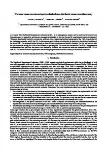
Fig. 1. Some basic channel types in Reo

Fig. 1 shows some example channels, whose semantics appear in Section 3. At this stage, we give an informal description of their behaviour. Sync denotes a synchronous channel. Data flows through this channel if and only if it is possible simultaneously accept data on one end and pass it out the other end. SyncDrain denotes a synchronous drain. Data flows into both ends of this channel only if it possible to simultaneously accept the data on both ends. SyncSpout denotes a synchronous spout. Data flows out of both ends of this channel only if it possible to simultaneously take the data from both ends. LossySync denotes a lossy synchronous channel. If a take is pending on the output end of this channel and a write is issued on the input end, then the channel behaves as a synchronous channel. However, if no take is pending, the 3

write can succeed, but the data is lost. Observe that this channel has contextdependent behaviour, as it behaves differently depending upon the context — if it were context independent, the data could be lost even if a take was present. AsyncDrain denotes an asynchronous drain. Data can flow into only one end of this channel at the exclusion of data flow at the other end. AsyncSpout denotes an asynchronous spout. Data can flow out of only one end of this channel at the exclusion of data flow at the other end. FIFO1 denotes an empty FIFO buffer. Data can flow into the input end of this buffer, but no flow is possible at the output end. After data flows into the buffer, it becomes a full FIFO buffer. FIFO1 (x) denotes a full FIFO buffer. Data can flow out of the output end of this buffer, but no flow is possible at the input end. After data flows out of the buffer, it becomes an empty FIFO buffer. A write operation to an input node succeeds only if all (input) channel ends coincident on the node accept the data item, in which case the data item is written to every input end coincident on the node. An input node thus acts as a replicator. A take operation on an output node succeeds only if at least one of the output channel ends coincident on the node offers a suitable data item; if more than one coincident channel end offers suitable data, one is selected non-deterministically, at the exclusion of all others. An output node, thus, acts as a merger. A mixed node behaves “pumping-station” that combines the behaviour of an output (merger) and an input node (replicator).

Fig. 2. Replicator and Merger respectively

To accurately model the behaviour of Reo nodes, we make the merge and replicate behaviour inherent in Reo nodes explicit and, without loss of generality, model them using two additional primitive connectors: a replicator and a merger (Fig. 2). The replicator primitive captures the replicator behaviour of an input node whereas the merger primitive models the behaviour of an output node. Informally, data will flow through a replicator if it can simultaneously accepts data on its input end and pass it to its two output ends. A merger permits the simultaneous flow of data from exactly one of its input ends to its output end, at the exclusion of flow on its other input end, making a non-deterministic choice if required. The mixed node, A, depicted in Fig. 3(a) is expressed in terms of the nodes A1 , . . . , A5 that are connected with one merger and one replicator as shown in Fig. 3(b). Thus, all nodes in this paper will consist of at most one input channel end and at most one output channel end. The term context in the title refers to the pending I/O requests on a con4

A1

A

A2

A4 A3 A5

A

(a)

(b)

Fig. 3. (a) Reo Node (b) Node replaced by a merger and a replicator

nector’s boundary, that is, the context in which a connector is used at a particular instant in time. A channel (hence connector) is said to exhibit context dependent behaviour whenever the behaviour of the channel (hence connector) changes dramatically with changing context. We use the phrase synchronisation constraints to denote the (context dependent) synchronisation and exclusion constraints imposed on the flow of data by Reo channels, replicators, and mergers. We define a routing as a solution to some synchronisation constraints. It determines where the data should flow and should not flow. The details of how to actually perform the flow are not a part of the routing. This paper presents a technique for solving synchronisation constraints based on a connector colouring scheme. Context dependent synchronisation constraints are solved using an extended connector colouring which can propagate context information to channel ends to dictate their behaviour. Although Reo connector may look like electrical circuits and the synchronous channels may lead the reader to think of Reo connectors as synchronous systems (as in Esterel [5]), it would be wrong to equate Reo with either model. Although the precise implementation details are more involved, a Reo connector is executed essentially in two steps: (1) based on pending write/take, solve the synchronisation/exclusion constraints imposed by the channels of a connector to determine where data can flow; and (2) send data in accordance with the solution in step (1). The second step may not occur if no data flow is possible. In between steps (2) and (1), new write/take operations may be performed on the channel ends, or existing ones may be retracted. Not all of the connector needs to be involved in step (1) at the same time: FIFO buffers, for example, serve to divide connectors into synchronous slices which operate more or less independently. Reo is designed so that connectors will be deployed in a distributed setting, with components and Reo nodes assigned to various machines across the network. We do not require that channels are mapped in a way that follows the wires of the network, though our implementation will assume that channels could be laid out it such a manner. This means that the underlying implementation will follow the topology of a connector when performing communications, which in principle enables Reo to be used in situations of limited 5

connectivity, such as wireless sensor networks.

3

Basic Connector Colouring

The semantics of a Reo connector is defined as a composition of the semantics of its constituent channels and nodes. We illustrate Reo’s semantics through an example, in part to give an understanding of how Reo works, but also to motivate the upcoming notion of connector colouring. The connector in

Fig. 4. Exclusive router connector

Figure 4 is an exclusive router built by composing five Syncs, two LossySyncs and one SyncDrain. The intuitive behaviour of this connector is that data obtained through its input node A is delivered to exactly one of its output nodes F or G. If both F and G are willing to accept data, then the node E non-deterministically selects which side of the connector will succeed in passing data. The SyncDrain and the two Syncs in the node E conspire to ensure that data flows at precisely one of C and D, and hence F and G, whenever data flows at B. An informal, graphical way of depicting the possible data flow through the exclusive router is by colouring where data flows, as illustrated in Figure 5, where the thick solid line marks the parts of the connector where data flows and unmarked parts correspond to the parts where no data flows. This idea of colouring underlies our model. Note that we abstract away from the direction of data flow, as the channels themselves determine this.

Fig. 5. Possible data flow behaviour. The thick solid line marks the part of the connector where data flows synchronously. In unmarked parts no data flows.

6

3.1 Colouring

Our model is based on the idea of marking data flow and its absence by colours. Each colouring of a connector is a solution to the synchronisation constraints imposed by its channels and nodes. Let Colour denote the set of colours. A reasonable minimal set of colours is Colour = { , }, where the colour ‘ ’ marks places in the connector where data flows, and the colour ‘ ’ marks the absence of data flow. Reo semantics dictates that data is never stored or lost at nodes [2]. Thus, the data flow at one end attached to a node must be the same as at the other end attached to the node. Either data will flow out of one end, through the node, and into the other end, or there will be no flow at all. Hence, the two ends plugged together will be given the same colour, and thus we just colour the node. Colouring nodes determines the colouring of their attached ends, which in turn determines the colouring of the connector, and thus the data flow through the entire connector. Colouring all the nodes of a connector, in a manner consistent with the colourings of its constituents, produces a valid description of data flow through the connector. Channels and other primitive connectors then determine the actual data flow based on the colouring of their ends. The following definition formalizes the notion of a colouring. Let Node be a denumerable set of node names. Definition 1 (Colouring) A colouring c : N → Colour for N ⊆ Node is a function that assigns a colour to every node of a connector. 2 Let’s consider a FIFO1 with input end n1 and output end n2 . One of its possible colourings is the function c1 : {n1 7→ , n2 7→ }, which describes the situation where data flows through the input end n1 and no data flows through the output end n2 . Channels, nodes, and connectors typically have multiple possible colourings to model the alternative ways that they can behave in the different contexts in which they can be used. The collection of possible colourings of a connector is represented by its colouring table. Definition 2 (Colouring Table) A colouring table, T, over nodes N ⊆ Node is a set of colourings with domain N . 2 Colouring a connector involves composing the colourings of its constituents so that they agree on the colour of their common nodes. To capture this notion, we define the binary operator, ‘·’, called join, which combines colouring tables.

7

Definition 3 The join of two tables T1 and T2 , denoted T1 · T2 , is defined: . T1 · T2 = {c1 ∪ c2 | c1 ∈ T1 , c2 ∈ T2 , n ∈ dom(c1 ) ∩ dom(c2 ) ⇒ c1 (n) = c2 (n)}. Here ∪ is the set-theoretic union on the graphs of the functions involved. The result is a function due to the side condition. The join operation satisfies the following useful properties, where 1 = {∅} is the colouring table with an empty colouring and 0 = ∅ is the empty colouring table. These properties are straightforward to prove. Proposition 4 Given colouring tables T , T1 , T2 , T3 then (1) (2) (3) (4) (5)

T1 · (T2 · T3 ) ≡ (T1 · T2 ) · T3 T 1 · T2 ≡ T 2 · T1 T 1 · T1 ≡ T 1 T ·1≡1·T ≡T T ·0≡0·T ≡0

(associativity) (commutativity) (idempotency) (unit) (zero)

A consequence of these properties is that “join” operation can form the basis of a distributed algorithm: associativity and commutativity allow colouring tables to be computed in any order, and idempotency enables the smooth handling of redundantly computed information, such as when two different concurrent computations of a colouring reach the same part of a connector.

3.2 Primitives A colouring table for a Reo connector describes the possible behaviour in a particular configuration (or snapshot) of the connector, which includes the states of channels, plus the presence or absence of I/O requests. A colouring corresponds to a possible next step based on that configuration. We choose as primitives: channels, mergers and replicators, and I/O operations. Definition 5 (Primitive) A primitive is a labelled tuple (nj11 , . . . , njkk )c , where for 0 < l ≤ k, nl ∈ Node, jl ∈ {i, o}, k ≥ 1 is the arity of the primitive, and c is its name, such that a node n appears at most as ni and no in (nj11 , . . . , njkk )c . A primitive with colouring is a pair of a primitive with a colouring table T over the nodes of the primitive. 2 The labels i and o indicate the direction of the end which is connected to node n. For example, (ai , bo )Sync denotes a Sync whose first end is an input end connected to node a, and whose second end is an output connected to node b. A colouring table for this primitive has colourings with domain {a, b}. Labels i and o help ensure that connectors are well-formed (Definition 6). We often omit such labels, tacitly assuming the well-formedness of connectors. 8

I/O operations: For each I/O request, a primitive colouring is used to denote whether it will be performed or delayed. We model the presence of an I/O request as primitive (nj ) and its absence as (nj ) , where j ∈ {i, o}. . . The colouring tables for these primitives are T = {{n 7→ }} and T = {{n 7→ }, {n 7→ }}, depicted graphically as and , respectively. The colouring tables T and T model the way components and connectors interact. T captures possibilities when no I/O operation is requested on a node by a component: no data flows through that node. T captures the possibilities when a data flow request is made by a component: either the data will flow or the connector will not allow it to do so. I/O operations need to be modelled in colouring tables so that we can determine the context dependent behaviour of a connector. It is the presence and absence of I/O operations on the boundary of a connector which gives the context. Replicators and Mergers: The behaviour of replicators and mergers is dictated by the semantics of Reo nodes. Their colouring tables are given in Figure 6. A replicator connector, (ai , bo , co )Rep , only allows data to flow synchronously Colouring Table

Replicator

a

a

b

c

Merger

c

b

Colouring Table b

a

c

a

b

c

b

a

c

Fig. 6. Colouring tables of a Replicator and a Merger

through all of its ends or none at all. When data flows, the data is replicated from a to b and c. A merger connector, (ai , bi , co )M er , allows data to flow synchronously from either a to c or from b to c with the exclusion of data flow at the other end. If both alternatives are possible, one is selected nondeterministically. Channels: Figure 7 presents the colouring tables for a selection of channels. We include an entry for both the empty and full states of the FIFO1 . As each 9

channel has two ends which are connected to nodes, there are two colours (which may be identical) for each channel colouring. Channel type

Sync

SyncDrain

SyncSpout

FIFO1

LossySync

AsyncDrain

AsyncSpout

FIFO1 (x)

Colouring Table

Channel type

x

Colouring Table

Fig. 7. Channels and their Colouring Tables

Channels that are completely synchronous, such as Sync, SyncDrain, and SyncSpout, have the property that either data flows synchronously at both of their ends or no data flows—abstracting away from the direction of data flow. Data flows from one end to the other through the Sync, flows into both ends of a SyncDrain, and flows out of both ends of a SyncSpout, as indicated by the arrows in the diagrams. The LossySync permits data to flow either all the way through the channel, or just at its input end (in which case, the data is lost), or no data flow. (This is not the whole story. We revisit this channel in Section 4.) The asynchronous channels, AsyncDrain and AsyncSpout, permit data flow at one end at a time only or no data flow at all. The data flow direction is analogous to their synchronous counterparts. An empty FIFO1 can accept data on its input end. A full FIFO1 can deliver data out of its output end. The other ends of these channels permit no data flow. 3.3 Connectors A connector is a collection of primitives composed together, satisfying some well-formedness conditions. As such, the colouring table of a connector is computed from the colouring tables of its constituents. Definition 6 (Connector) A connector C is a tuple hN, B, E, T i, where • N is the set of nodes that appear in E; • B ⊆ N is the set of boundary nodes; • E is a set of primitive connectors; 10

• T is a colouring table over N ; such that: (1) n ∈ B if and only if n appears only once in E; and (2) n ∈ N \ B if and only if n occurs once as no and once as ni in E. 2 A primitive with a colouring table can straightforwardly be considered as a connector. A connector’s semantics is computed by joining the tables and other elements of its constituents: Definition 7 Let C1 = hN1 , B1 , E1 , T1 i and C2 = hN2 , B2 , E2 , T2 i be connectors such that (N1 \ B1 ) ∩ (N2 \ B2 ) = ∅, and for each n ∈ B1 ∩ B2 , ni appears in E1 and no appears in E2 , or vice versa. The join of C1 and C2 , is given by: . C1 C2 = hN1 ∪ N2 , (B1 ∪ B2 ) \ (B1 ∩ B2 ), E1 ∪ E2 , T1 · T2 i. 2

3.4 Example

We illustrate the process of computing the colouring table of a connector from its primitives by means of an example. To simplify the presentation, we omit some details which the diligent reader can easily fill in. Let’s consider the connector: n1

n3

n2

n4 .

Denote the channels as C1 , C2 , and C3 : C1 = h{(n1 , n2 )Sync }, T1 : {{n1 7→

, n2 7→

C2 = h{(n2 , n3 )AsyncDrain }, T2 : {{n2 7→ {n2 7→

, n3 7→

}, {n1 7→

, n3 7→

, n2 7→

}, {n2 7→

}}i

, n3 7→

},

}}i

C3 = h{(n4 , n3 )Sync }, T3 : {{n4 7→

, n3 7→

}, {n4 7→

, n3 7→

}}i.

The crux of computing C1 C2 C3 is computing the underlying table: T1 · T2 · T3 . Now, T1 · T2 = { {n1 7→

, n2 7→

, n3 7→

},

{n1 7→

, n2 7→

, n3 7→

},

{n1 7→

, n2 7→

, n3 7→

}}.

11

Continuing, (T1 · T2 ) · T3 = { {n1 7→

, n2 7→

, n3 7→

, n4 7→

},

{n1 7→

, n2 7→

, n3 7→

, n4 7→

},

{n1 7→

, n2 7→

, n3 7→

, n4 7→

}}.

We can graphically depict the colouring table just computed as: n1

n2

n3

n4

n1

n2

n3

n4

n1

n2

n3

n4

Indeed, this is the preferred way of presenting colouring tables, because they give a pictorial representation of the data flow in a manner which follows the shape of the connector. By adding an I/O request to the boundary nodes of the connector just computed, we have enough context information to determine how the connector can route data. The following are the two possibilities when there is an I/O opearation (write) on node n1 and no I/O operation on node n3 : n1

n2

n3

n4

n1

n2

n3

n4

The first entry in the colouring table describes successful data flow. The second entry describes the total absence of data flow. In this example, only the first entry would be allowed. The latter possibility is not desirable, because there is no data flow, although there is no reason to prevent data flow. This is caused partly because connector colouring is not sensitive to the context in which a connector appears. We shall see in the next section that this problem can be worse, as it arises not only at the boundary of a connector, but also when channels exhibiting context dependent behaviour appear in the middle of connectors—how can they determine the context in order to behave correctly? In Section 4 we extend our colouring scheme to accurately describe context dependent behaviour and to propagate it through connectors. In the remainder of the paper, we refer to the present colouring scheme as 2-colouring and the extended one of the next section as 3-colouring. 12

4

Context Dependent Connector Colouring

In this section we address the issue of context dependent behaviour. We demonstrate that the 2-colouring scheme applied to a connector involving a LossySync fails to give the expected data flow behaviour. We observed a similar situation in the example at the end of Section 3.4. We argue that this occurs because context information is not propagated to enable channels to choose their own correct context dependent behaviour. Previous semantic models of Reo connectors [3,6] remain at a coarser level of abstraction and fail to address this issue. A LossySync has the following context dependent behaviour (as described in Section 2). If both a write is pending on its input end and a take is pending on its output end, then it behaves as a Sync—the write and take simultaneously succeed, and the data flows through the channel. If, on the other hand, no pending take is present, then the write succeeds but the data is lost. Problems with the 2-colouring scheme reveal themselves when we compose a LossySync, an empty FIFO1 , and an I/O request on the input end of the LossySync, as follows: a

b

c

.

This connector has the following two alternative 2-colourings: a

b

c

a

b

c

.

The first colouring indicates that the I/O operation succeeds, the data flows through a and that the LossySync acts as a Sync sending the data through b into the FIFO1 . This is the expected behaviour in this configuration. The second colouring indicates that data flows through node a, but not at node b, indicating that it is lost in the LossySync. An empty FIFO1 is, however, input enabled, meaning that it should always be able to accept data. Another way of seeing this is that an empty FIFO1 always issues a take to whatever channels it is connect to. Indeed, the only reason that it should not succeed in receiving data is if the connector gives it a reason not to—such as by not sending it any data. One can therefore interpret the situation as a violation of the intended semantics of the LossySync channel, because the information that the data can be accepted on its output end is not appropriately propagated to it. The LossySync cannot detect the presence of the pending take issued by the input-enabled, empty FIFO1 buffer. Similar situations arise when dealing with a LossySync in isolation or in the context of any connector. The behaviour of a context dependent primitive depends upon the presence or absence of I/O requests on its ends. For mixed nodes, however, no I/O request 13

information is present, so it is not obvious what the context is. The key to resolving this is to determine what context information can be consistently propagated while addressing synchronisation constraints. Rather than propagating the presence of an I/O request, our approach focuses on propagating their absence, or more generally, on any reason to delay data flow, such as unsatisfiable synchronisation constraints or due to choices made by a merger. In the next section, we present the 3-colouring scheme which uses colourings to propagate “reasons to delay”. Using this scheme, the undesirable colouring for the LossySync-FIFO1 connector described above can be ruled out due to the mismatch of colours at node b, as follows:

a

b

c

.

This means that the possibility of losing data in the LossySync is no longer a behaviour of the LossySync-FIFO1 connector.

4.1 Trois Couleurs: Reo

To address the problem just described, we modify our set of colours. Since we wish to trace the reason to delay, we replace the no-data-flow colour by two colours which both use a dashed line marked with an arrow. The arrow indicates the direction that a reason to delay comes from, that is, it points away from the reason in the direction that the reason propagates. Thus we , }. In fact, the colours depend now work with colours, Colour = { , upon how the arrow lies in relation to the channel end being coloured. A no•, means give a flow colouring with the arrow pointing towards the end, reason to delay, and a colouring with the arrow pointing the opposite way, •, means require a reason to delay. 3 We can compose two colourings at a given node if at least one of the colours involved gives a reason to justify no flow. Of the four possible combinations of end colourings at a node, three can compose, as given in the following table:

3

To be precise, the colours also depend upon the direction of data flow. Giving a reason on an input end is the same colour as requiring a reason on the output end, and giving a reason on an output end is the same colour as requiring a reason on the input end.

14

•

X

•

X

•

X

•

×

The last case is not permitted as it joins two colouring which require a reason to delay, without actually giving a reason. Note that after composition has been performed, the direction of the arrow on mixed nodes no longer matters: the colouring simply represents no data flow. (This fact is used to reduce table sizes.) A problem with 3-colouring is that tables usually contain redundant entries. The following principle, the flip rule (Definition 8), reduces tables to their essential colourings. It can be used as a guide for constructing tables for primitives, and it is also used in the implementation to reduce table sizes. Definition 8 (The Flip Rule) If colouring table T has an entry c which maps boundary node n to the colour •n , that is, giving a reaons, then the colouring which is the same as c except that n is mapped to • n , that is, requiring a reason, is redundant and can be removed from the table. The rationale behind the flip rule is as follows. Consider two colourings in a table that differ only in the colour of node n; that is, one colouring has •n , the other has •n . These two colourings can both compose with a colouring containing colour •n . The resulting colourings have no flow at node n, but are otherwise identical. Removing the colouring containing •n from the table does not reduce the table’s composibility with other tables. On the other hand, removing •n does reduce composibility. So the colouring containing •n is superfluous, whereas the one containing •n is not. Observe that the flip rule applied to any table T induces a lattice. Denote the largest element, the one with the most redundancy, as T + . In addition, the flip rule induces an equivalence class on tables (take the symmetric, transitive closure of the lattice), which we denote ≡. A minor problem remains. The notion of composition given so far is not compatible with the definitions from Section 3, as is not based plugging together matching colours. We can define a second notion of composition which excludes the third entry from the composition table above and applies to maximal tables (T + ). This notion is compatible with previous definitions. Furthermore, the two notions are equivalent in the following sense. Let ·1 denote the first notion and ·2 be the second notion. 15

Proposition 9 Given tables T1 and T2 which can compose. Then: T1 ·1 T2 ≡ (T1+ ) ·2 (T2+ ). This means that we can use whichever notion of composition is most convenient and that we can think in terms of tables compressed using the flip rule. The colourings for all primitives will now be redone. IO operations: An I/O operation primitive has the following colouring table: Colouring Table

I/O (present/absent) /

The second entry indicates that the I/O operation request is delayed because the connector gives a reason to prevent it. The third and fourth entries indicate that no I/O operation request is present, hence no data flow is possible. Furthermore, the third entry states that the absence of I/O can be used to justify a delay. The fourth entry represents the case where the reason to delay is already present in the connector. The one possible case missing from this table, like the second case with the arrow going the other way, does not make sense. It would read: there is an I/O request which is a cause of delay. This case is therefore omitted. Using the flip rule, the colouring table for the I/O primitive can be replaced by the following: Colouring Table

I/O (present/absent) /

The flip rule can be used to recover the missing entry, yielding the fourth (above) from the third. From now onwards, we always use tables that are reduced by application of the flip rule. Replicators and Mergers: We update the colouring tables for mergers and replicators. The diligent reader may demonstrate by herself that the flip rule accounts for all other sensible possibilities—doubling the table size in each case. The new colouring table for a replicator is: 16

Replicator

Colouring Table

The last three entries indicate situations where no data can flow. In each case, a reason to delay coming from one end is sufficient to cause delay in the entire replicator. The reason for delay is propagated to the other ends. The new colouring table for a merger is: Merger

Colouring Table

The first two entries in the table deal with choices made by the merger. Data flowing down one input branch is sufficient reason to delay data flow in the other input branch. The third entry corresponds to no take being present at the output end: no data flow is possible in the merger, and the reason to delay is propagated to the input ends. The final entry corresponds to no data flow due to no data availability at either of the two input ends. Again the reason to delay is propagated. Note that neither colouring table includes an entry with all arrows pointing outward. This would indicate that the reason came from nowhere. Channels: The new colouring tables for channels are given in Fig. 8. The colouring , for example, is shorthand for the colouring , which means that the reason for delay is propagated from one end of the channel to the other. We highlight a few points of interest in this table, focusing only on reasons to delay, leaving the reader to ponder over the rest. Failure at one end of a Sync, SyncDrain or SyncSpout, is enough to prevent data flow. The reason is propagated to the other end. An empty FIFO1 buffer does not enable data flow on its output end, giving a reason for delay. Dually, a full FIFO1 buffer has a reason to delay its input end. The second entry of the table for a LossySync states that it will lose the data only when a reason to delay is propagated into its output end, which amounts to saying that the 17

Channel type

Sync

SyncDrain

SyncSpout

FIFO1

LossySync

AsyncDrain

AsyncSpout

FIFO1 (x)

Colouring Table

Channel type

x

Colouring Table

Fig. 8. 3-Colouring Tables for Channels

channel is unable to transfer the data. For the two asynchronous channels, AsyncDrain and AsyncSpout, accepting data on one end is sufficient reason for delaying the other end. No data flows if both ends have a reason to delay. Note that a non-deterministic choice may be required to decide between the first two possibilities.

4.2 Example In this example, we introduce a new primitive, a priority merger, and use it to model a priority router. A priority merger behaves similarly to a merger, allowing flow of data from at most one of its input ends to its output end. The difference is that whenever data is available on both of its input ends, such as when there is a write pending on both ends, then the channel gives priority to a specific end (marked with an exclamation mark ’ !’). The graphic representation and the colouring table for the priority merger are presented in Fig. 9. Compare the first two entries in the table. The first entry means that allowing flow in the right input can give a reason to delay the left input. On the other hand, the second entry means that data can flow from the left input only if a reason is given on the right input. This reason could be that no data flow is possible on that input. Let’s now construct a priority router. This behaves like an exclusive router, except that rather than making a non-deterministic choice when two takes are pending, it makes a choice dictated by the priority merger primitive. The priority router is given in Fig. 10, along with the only 3-colouring possible in the configuration where I/O requests are present on all of its ends. This means that in the presence of two competing takes on the output ends of the 18

Colouring Table

!

Priority Merger

Fig. 9. Priority merger connector and its 3-colouring table

connector, the left hand one (which has priority) will always succeed. This is because the colouring table of the priority merger (appropriately rotated), in the presence of the I/O requests, cannot give a reason for the left hand branch to delay, though it can give a reason for the right hand branch to delay. Priority Router

Colouring

! Fig. 10. A Priority Router and a colouring exploiting context dependency.

We recall now the example in Section 3.4 and the case of the LossySyncFIFO1 connector presented in the beginning of this section. In both cases we can see that the respective 3-colourings of the undesirable alternatives are now impossible. In the first example (from § 3.4), the colours do not match on node n2 : n1

n3

n2

n4

In the LossySync-FIFO1 example, the colours do not match on node b:

a

b

c

.

These examples illustrate how the propagation of I/O context in the 3-colour setting can be used to resolve the context dependency constraints on the priority, I/O operations and LossySync channels. Note however that priority is not globally decided. It may be the case that a decision made by a different part of the connector makes priority irrelevant or even inverts the decision—it all depends upon the connector. 19

4.3 Causality Loops

The model presented thus far still produces incorrect colourings for some connectors containing loops. Colourings for synchronous loops in a connector tend to result in so-called causality loops. These occur whenever a chain of causeeffect events is circular, giving, for example, a colouring that corresponds to data flow being present, but for which there is no source of data. The anomalous behaviours are a standard problem in synchronous languages [5]. In our setting the problem is somewhat more complicated, because, not only do we need to consider causality loops which concern data flow, but also causality loops concerning reasons for delay. Both kinds of loops need a source of either data flow or reason to delay to be valid, depending on the kind of loop. Fig. 11 illustrates the two kinds of loop: (a) a loop for which the colouring states that data can flow, even though there is no source providing data: where does the data flowing at C come from? and (b) a loop for which the colouring states that there is a reason for delaying, even though there is no source providing a reason: where does the reason to delay observed at A come from? Causality Loop

Connector (a) B

A

B

A

C

C

(b) B

A

B

A

C

C

Fig. 11. Causality Loops in Two Reo Connectors. In (a) the loop follows the data flow of the channels. In (b) the loop follows the reason to delay arrows.

The basic approach to finding causality loops is to trace all paths backwards in causality graph to see whether there is, in our case, an actual source of data or delay. Various solutions have been proposed to treat causality loops [7]. These solutions can be adapted to compute in a compositional manner that every path in a colouring has a proper source, where (a) in a solid colouring, the path is given by the direction of the data flow and the source is a source of data, and (b) in a no-flow colouring, the path is given by the direction of the arrows and a source is a reason to delay. 20

Observe that causality loops are reasoned about at the level of individual colourings; other valid colourings for the connectors may be possible. Removing colourings that contain causality loops from colouring tables results in a more sensible semantics for Reo connectors, as colourings which correspond to anomalous situations are removed.

5

Implementing Connector Colouring

In this section we discuss how connector colouring forms the basis of a nondistributed implementation of Reo connectors, and how it can be extended to a distributed implementation based on CWI’s MoCha mobile channel middleware [8]. Before presenting the details, we outline some requirements that a distributed implementation ought to satisfy. We then present the general kind of scheme which we anticipate that algorithms implementing connector colouring will follow. The non-distributed implementation, called Reolite, which implements most of the original Reo proposal, is described. A distributed algorithm for connector colouring based on spanning trees is presented.

5.1 Requirements for Implementation of Reo A distributed implementation of Reo must fulfill the following requirements: No Global View In a geographically distributed environment, different parts of a Reo connector may reside on remote hosts. A global view of a connector’s state can result in single point-of-failure vulnerability, and the delays necessary for maintaining a consistent global view may inhibit the parallelism inherent in physically distributed systems. Without a global view, the constituents of a connector have only a limited knowledge about the connector, and must delegate requests to other parts of the connector in order to obtain the information required to transport data. Communication Infrastructure and Topology In Reo, channels encapsulate all communication-related activities. Since channels provide the only infrastructure for communication, only the paths defined by the interconnection of channels, the connector topology, can be used to send the control information required to determine the data flow of a Reo connector. Propagation of Synchronisation Constraints Reo channels and nodes impose synchronisation and exclusion constraints on data flow across the entire connector. Data flows atomically through the “synchronous” parts of a connector. The state of the entire connector and its boundary may be required to determine how data can flow. One approach to determining the flow of data is to optimistically send 21

data along channels and rollback any changes when synchronisation constraints cannot be met. Aside from requiring a rollback capability on every channel, which may not be feasible in practice, this approach may, in general, result in too much wasted resources or network flooding trying to find a suitable data flow. The alternative preferred here is to pre-compute the routes of possible data flow, and then, non-deterministically choose one to take, whenever required. Concurrency In a distributed environment, multiple parties may interact with a connector at the same time. This means that more than one computation to determine a connector’s data flow can be active, leading to a situation where different computations are competing for parts of the connector. Without proper handling of these situations, these concurrent data flow computations can face race conditions, livelocks, deadlocks, or simply waste resources.

5.2 Algorithm Scheme

Any algorithm using connector colouring as the basis for deciding how to route data through a Reo connector will need to perform the following steps, though not necessarily strictly in the order presented. We assume that the configuration of a connector including its pending I/Os is locked when the colouring table is computed, although at any other time parties may delay, timeout, retry, and new parties may join—changing the configuration of the connector and its environment. (1) Compute colouring table for complete connector: Collect all the colouring tables from all the channels and inputs and outputs for the connector. Compute the composite colouring table. (2) Select route to employ: The computed colouring table may contain 0, 1 or many colourings. If the table has no elements, no communication occurs. If the table has one element, then that is selected. Otherwise, select a colouring non-deterministically. (3) Distribute the chosen colouring to all parties: The chosen colouring is distributed to all parties so that they have a consistent view, according to the synchronisation constraints, of what the data flow will be. (4) Send data: Each data source (write/FIFO1 buffer) which has been selected to have data flow can send its data as soon as it gets the final colouring table. All choices that a primitive needs to make are determined by the chosen colouring. A number of variations are possible. Rather than globally computing the table, it could be computed using a parallel algorithm such as all-reduce [9]. If 22

the local tables are T1 , . . . , Tn , reduce computes T1 · T2 · · · Tn ; the all part corresponds to sending this information to all parties. In practice one does both steps together, relying on the properties of the operator ‘·’. To deal with the case that multiple entries are possible, simply order the entries in the table and choose the first. Entries should be placed in the table non-deterministically for fairness. Alternatively, some form of negotiation might be required to choose a colouring. This falls into the class of problems known as reaching consensus in a distributed network [10]. We now will describe how connector colouring is implemented in Reolite.

5.3 Reolite: A Non-Distributed Reo Implementation

Reolite [11] is a non-distributed, connector colouring-based, Java implementation of most of Reo, as described in Arbab’s original article [2]. 4 Reolite is a rudimentary proof-of-concept to demonstrate the feasibility of connector colouring compared to the previous approach based on accepts and offers [2,12].The previous approach to implementing Reo was so complex that it cost approximately a man year of effort to implement a system which neither worked particularly well nor was easy to reason about. Based on connector colouring, Reolite was up and running within a fortnight. Reolite permits a number of components, running their own threads, to interact with a connector, which itself is managed globally by a single thread. Interaction occurs only between a component’s thread and the connector whenever a component attempts to write to or take from a channel end. The connector is protected by a global lock, which means that whenever the connector thread is calculating the colouring table or performing data flow, the connector cannot be changed—even registering a new pending write or take is impossible. The interaction between a component and the connector is best described by detailing the two kinds of thread. Note that this locking scheme is too coarse grained to be scalable, but it works well for the proof-of-concept. Component Thread Whenever a component performs a write or take on a channel end, it begins interacting with the connector as follows: (1) start timer for timeout (2) obtain connector lock 4

Lacking are operations for connecting components to and disconnecting components from connectors, and for moving nodes, as these have no effect on the connector behaviour, the hiding construct, and channels which are data sensitive, such as a filter.

23

(3) if writing then register that data is being written to the channel end if taking then register that data is requested from the channel end (4) release connector lock (5) notify connector and block (6) when awoken if awoken by connector (assumption: this end was chosen in a colouring) kill timer return, with data if operation was a take if awoken by timeout obtain connector lock if write/take has since succeeded release connector lock return, with data if operation was a take else deregister write/take release connector lock throw timeout exception Note that a timeout will never occur if the connector is busy, to avoid resulting in inconsistency across the connector. Thus it may be the case that a timeout expires (under the hood), but that data is nevertheless returned. Connector Thread (1) obtain connector lock (2) collect colourings from all channels and input and output ends (both those which have pending operations and those which do not). (3) compute colouring table (4) select a colouring (5) loop select a source of data which is coloured pass its data into approriate channel, which may create new sources of data reset input and output ends which have had their request satisfied remove such ends from colouring until data has flowed at all coloured ends (6) release lock. Channels have data pushed into their input end(s). This data will appear at any output end(s) based on the channel’s implementation in accordance with the colouring selected for the channel (otherwise the channel is not correctly implemented). In addition to this algorithm, the connector periodically gains control and performs any actions that it can—this is necessary to, for example, push data 24

through chains of FIFO1 buffers. The implementation of Reolite also enables dynamic reconfiguration of connectors (using join and split [2]), and permits channel ends to be passed through connectors, enabling complex dynamic coordination patterns. New components can be added to an existing system, assuming that the connector first knows the name of one of the channel ends. This deficiency has been removed in MoCha [8], which permits the advertisement and discovery of channel end names.

5.4 Distributed Algorithm — Single Party Version We now present an informal description of a somewhat idealised version of the distributed algorithm, which is presently being implemented and tested. We do not address issues of fault tolerance. Full details of this work included a proof of correctness will be reported in future work. The algorithm which follows may be initiated at any input or output node by an I/O request, or by a buffer trying to forward its data. In addition, the algorithm may be concurrently initiated at different nodes by different parties. We first describe the algorithm from the perspective of one such party, assuming that no interference with other parties occurs. Then, in the next subsection, we describe how to deal with multiple parties computing concurrently. The algorithm follows the topology of the connector using remote procedure calls rather than message passing. Calls traverse the graph of a connector by passing from a node, to the channel ends forming the node, then to a channel, which may propagate the call to their other end, and then to some node again. Information describing the state of the algorithm may be stored in channel ends. The initial state is Sleeping. The first phase of the algorithm is called collect. It proceeds as follows. Starting with the initiating node as root, a spanning tree of the connector is formed. This is achieved simply by traversing the graph of the connectors, marking each channel end as it is visited (state Collect), ceasing further progress whenever an already visited end is met. The forward leg of this phase thus traverses a spanning tree of the Reo connector. The return leg collects the colouring tables of each channel and node. The complete colouring table is then computed at the root, and an entry of the table is chosen. The algorithm then enters the second phase, called propagate, in which the chosen colouring and the data to be sent are propagated through the connector. The interesting behaviour occurs on channel ends, and there are essentially three cases to deal with: 25

(1) For calls following the direction of data flow where the channel end is coloured, the colouring is passed onwards (through channel or through node) along with the data. On the return leg, the state is reset to Sleeping. (2) For calls against the direction of data flow where the channel end is coloured, the colouring is passed onwards, and on the return leg, the data is returned and the state is reset to Sleeping. (3) For calls where there is no data flow, the colouring is propagated, potentially to places where flow is possible, and the state is immediately reset to Sleeping. Nodes get data from any coloured output end and propagate it to any coloured input end. Channels accept data from coloured input ends, process it whatever manner they see fit, so long as it is consistent with the selected colouring, and forward data on their coloured output ends. At the end of this phase, data will be passed through the connector as described by the colouring, and the transient state stored by the algorithm in the channel ends will be reset to its initial state. 5.5 Distributed Algorithm — Multiparty Version We now outline a distributed algorithm in which the computation described above is initiated in multiple parts of the connector. The first thing to note is that the colourings enable one to consider different computations to be cooperatively computing the same global colouring scheme, which is in contrast to Internet routing algorithms where packets compete for passage through the network [13]. This means that any partial table computations can be combined, potentially reducing work. The second thing to note is that we assume a global ordering on the channel end names. Although this is a theoretically difficult issue, a number of ways exist for doing this in practice, such as basing the name of a machine’s network card’s MAC address, the IP number, and/or the active thread’s pid. As above, every channel end stores state information used by different threads to determine what the other threads are doing. Initially, all threads are in the Sleeping state. State Collect denotes that the end has passed in the collect phase—this state stores also data indicating the id of the initiating thread. Finally, the state Propagate indicates that the algorithm is propagating colouring and potentially data information—this state stores the colouring table, the direction of propagation (against or with the flow of data) and the data value (if available). When an end is passed by the collect phase, the algorithm marks the end with 26

state Collect and the id of the initiating end. If the collect phase passes an end which is marked with the same state, it knows that it has hit a loop and it starts returning the collected results. If it passes an end in state Collect with another id, then the thread with the highest id continues, and the thread with the lowest id backs off. Otherwise, it continues constructing the spanning tree—it can stop prematurely if it detects that it has completed the colouring. If a collecting thread passes an end which is in the middle of propagating data (state Propagate), then it also backs off. Whenever a computation backs off, it waits until the initiating end is reset to the Sleeping state. The computation will then be retried if the associated I/O request has not been satisfied. When an end is passed by the propagate phase and the end is in state Collect, the progagate algorithm continues as normal, setting the state to Propagate (with the direction, colouring table, and any data stored too). If the node is in the Sleeping state, it means that another thread of the propagate phase has passed this way, so this thread returns—the data that it needs to propagate will be stored by another thread in one of the ends previously visited by this thread. If the propagate phase passes an end in state Propagate, it does one of two things. If this thread has data, it writes the data into the state on the end and returns. If this thread is waiting for data, it suspends until the end receives data from some other thread. In all cases, at the end of the propagate phase, ends states are set back to the original Sleeping state.

5.6 Discussion

The complexity of sending data though a Reo connector depends upon two factors: the size of the synchronous slice—a part of the connector not separated by FIFO buffers—and the size of the colouring table, which is a function of the size of the synchronous slice. Assume that there are n channel ends in a synchronous slice. The algorithm then, in the worst case, passes sequentially through these n ends. Assume that the size of the accumulated is T (n). It is clear then that the complexity of the algorithm is O(n × T (n)) for each data item that needs to be sent. In the worst case the table is exponential in the size of synchronous slice, so the algorithm has exponential complexity. Often table sizes tend to be linear in n, and thus the overall complexity is O(n2 ). The fact that table sizes can be large tended not to be a problem in our limited experience. Table sizes reduced after a number of additional optimizations were implemented: (1) tables are stored as sets, rather than lists, to avoid duplication; (2) all internal “no-flow” colours have their arrows removed, since the direction of the arrow matters only on the boundary—this unifies many possible table entries; (3) the flip rule is used to avoid duplication in the 27

table (Definition 8); and (4) some causality loops are detected and removed (Section 4.3). Combined these optimisations reduced the size of the colouring table for the exclusive router from over 1000 entries to just the expected 4. The high complexity of the algorithm is due to Reo, rather than the algorithm itself. But there are a number of additional ways of managing the complexity. Firstly, avoiding deploying synchronous slices across different machines helps localise the cost. Making connectors less synchronous is another way, but this means using a different connector. Ultimately, the trade-off between degree of synchronisation and acceptable performance can only be determined through benchmarking various candidate connectors. The algorithm works in the setting where each party knows nothing of its neighbours, except how to find them (via the topology of the connector). Different parties can compute concurrently, though the topology of the connector may limit how much concurrency can be exploited in computing a colouring table. The colouring table is computed as a solution to the synchronisation constraints before any data flows, rather than optimistically sending data which would need to be retracted or ignored. Although the colouring table is completely obtained in one node (of a synchronous slice), we argue that the algorithm still satisfies the no global view constraint, as the algorithm need not maintain this view. It simply uses it to perform a step. We argue, thus, that the algorithm satisfies the 4 criteria presented at the start of this section. There are two other issues to consider: dynamic changes in a Reo connector and partial failure of the network. Dynamic changes to a Reo connector, such as reconfiguration, can be catered for, as these must observe the locking scheme and can only occur when the node being modified is in the Sleeping state. Some of the algorithms for recofiguration and mobility implemented in the MoCha middleware [8] can be adapted to our setting. The main point where the algorithm suffers is dealing properly with partial failure. Put simply, the algorithm doesn’t deal with partial failure. But it is possible to deploy a connector so that it does not suffer from problems of partial failure, by by ensuring that no synchronous slice of a connector spans multiple machines in a network.

5.7 Summary of Implementation Status

We have a running non-distributed version of the colouring algorithm [11] with GUI support for connector drawing and connection with Unix processes [14]. Work is being undertaken to extend this to work with Web Services. A prototype version of the distributed algorithm has begun using Ruby and its 28

remote procedure call mechanism. This will serve as a suitable platform for benchmarking various approaches to implementing the distributed algorithm, as well as exploring issues such as deployment, before committing to a more difficult C++ implementation and integration with MoCha [8].

6

Related Work

Reo is capable of defining connectors with sophisticated behaviour using very few primitive channels [2,4,6]. Predecessors to Reo, namely MoCha [8] and Manifold [15], did not impose synchronisation constraints to the degree that Reo does, and hence were simpler to implement but less expressive. Reo enables synchronisation and exclusion constraints to propagate across a connector, whereas these models could not. Older coordination languages and models such Linda [16] and Gamma [17] cannot directly exhibit the degree of synchronisation that Reo can. This fact remains true for all of the coordination models covered in a recent survey [1]: Reo’s approach to coordination, in particular, to synchronisation and exclusion, is unique. The notion of connector is not unique to Reo, as it appears in the study of software architecture [18], and also in the guise of a coordination model for active objects [19]. The main distinguishing feature of Reo is that it enables the simple compositional expression synchronisation and exclusion constraints, whereas the other work on connectors focuses more on connecting behavioural interfaces of components. Both aspects are two pieces of the same pie. A number of informal and formal models exist for Reo. The first operational description of Reo [2] describes connector behaviour in the presence and absence of requests at channel ends in a context dependent manner. An operational model based on what values connectors offered and accepted proved, however, to be too difficult to reason about and to implement [12]. Semantic models based on a coinductive calculus [6] and on constraint automata [3] paved the way to reasoning about connectors and their expressiveness, and for the mechanical verification of their properties. These two models were proven equivalent under mild fairness assumptions. We will now expend some effort comparing connector colouring with constraint automata. One aspect of the constraint automata model is that transitions in automata are labelled with the collection of nodes that synchronously succeed in a given step, at the exclusion of all other nodes present in the connector being modelled. Calculating this set based on the configuration of a connector (which is equivalent to the state of the constraint automata) is precisely what connector colouring achieves. That is, the 2-colouring model of a connector produces a set colourings which can be equated with the transitions in the cor29

responding constraint automata. Our model has the novelty of being simpler, as it focuses on the key difficulty, namely determining which transition to take next, rather than worrying about what state that will lead to. Our model also has the advantage of being visually appealing, as the colouring can overlay the connector. Furthermore, the 3-colouring captures the context dependent behaviour of connectors, which other semantic models did not. Network algebra [20] provides a general framework for the study of networks and their behaviour. We expect that our work can be rephrased in this framework, which would enable a better comparison with various existing work. The recent work of Bruni et al [21] proposes a semantic model for CommUnity connectors, the core of which is a denotation for each primitive connector based on ticks and unticks corresponding to the presence and absence of data flow. This clearly is similar to our 2-colouring scheme, although we have both loops in our connectors and a larger set of primitives. As far as we are aware, these languages and formalisms do not have quite the range of expressiveness covered by the channels present in Reo, such as LossySync with its subtle behaviour, nor do they require or express context dependence, as we address in this paper. The synchronised hyperedge replacement approach [22] of modelling distributed systems using graph transformations has some similarities with Reo, in that the synchronisation is transitive across large chunks of the graph or connector. Transformations in a graph change the structure of the graph, whereas in Reo the structure of the connector is more static, though the internal states of buffers may change. Computation in a Reo connector is realised when data travels though a connector and its state changes, whereas the transformation of a graph is computation in the graph model. Milner’s classic SCCS [23] also appears to be an appropriate model for “implementing” our 2- and 3-colouring schemes, 5 by mapping colours to SCCS actions, after polarizing the ends joined at a node. For example, we could model the 2-colouring behaviour of a LossySync with ends connected to nodes named a and b as: . LossySync(a, b) = δ(Flow(a) × Flow(b) + Flow(a)) : LossySync(a, b)

Modelling the 3-colouring scheme of the same LossySync requires more than a simple use of the delay operator (δ). Actions need to be expanded to also include no-data-flow colours, in order to properly propagate the constraints they encode. One possible encoding of the LossySync is the following, which uses NoFlow(b) and NoFlow(b) to denote the giving and the requiring of a reason, respectively: 5

We thank an astute referee for this observation.

30

. LossySync(a, b) = ( Flow(a) × Flow(b) + Flow(a) × NoFlow(b) + NoFlow(a) × (NoFlow(b) + NoFlow(b)) ) : LossySync(a, b)

This approach to encoding Reo in SCCS is worth further investigation. Our model resembles the Tile Model [24]. Indeed, the Tile Model is a very general framework for the compositional description of transition systems. Our colouring and the semantics of Reo, including its reconfiguration operations, could very nicely fit within this model, though we do not know how well the Tile Model deals with loops in connectors. The key difference is that the Tile Model is a general formalism, whereas our connector colouring deals with the specifics of Reo. Colouring is a natural concept and appears in various contexts throughout the literature. For example, a variant of Petri nets called Coloured Petri Nets [25] exists. The different colours correspond to abstractions of various data values; thus colours are types or sorts. Colouring also appears in graph algorithms: these algorithms aim, in general, to colour different connected parts of the graph differently [26]. So, for example, a 3-colourable graph is one which each vertex can be assigned one of three colours so that no edge joins two equicoloured vertices. Both of these uses of colouring are distinct from ours. We believe that our 3-colouring scheme is new, and that it can form the basis for coordination models which enforce synchronisation and exclusion constraints in a manner that depends upon the way in which components are interacting with the coordination layer.

7

Conclusions and Future Work

We presented a model for Reo connectors based on the idea of colouring a connector with possible data flows in order to resolve its synchronisation and exclusion constraints. A more sophisticated notion of colouring enables the model to capture context dependent behaviour, which more closely matches the informal descriptions of Reo’s semantics [2] than earlier formal attempts [4,3]. Our model is easy to work with and its underlying “join” operation satisfies useful algebraic properties, making it a suitable basis for the distributed implementation of Reo. Such an implementation has the freedom to compute data flow possibilities concurrently, in a manner which is robust to redundancy, because multiple partial computations can be combined. Our work, thus, serves as a basis both for an implementation and for a more precise semantic model of Reo. 31

The present work has limitations which we intend to address in future work. It does not address all of Reo’s features: node hiding and data-sensitive behaviour, such as the filter channel [2], need to be added. There are two difficulties here: (1) it is unclear how to implement hiding to correctly preserve the desired observable behaviour of a Reo connector, especially in the presence of channels with context dependent behaviour; and (2) it is unclear how to handle data-sensitive channels efficiently.

Acknowledgements To Nikolay Diakov a very thorough reading of an earlier draft, and for providing important suggestions for Section 5, and to the members of SEN3 for enduring various presentations of this work.

References [1] G. A. Papadopoulos, F. Arbab, Coordination models and languages, in: M. Zelkowitz (Ed.), The Engineering of Large Systems, Vol. 46 of Advances in Computers, Academic Press, 1998, pp. 329–400. [2] F. Arbab, Reo: a channel-based coordination model for component composition, Math. Struct. in Comp. Science 14 (3) (2004) 329–366. [3] F. Arbab, C. Baier, J. Rutten, M. Sirjani, Modeling component connectors in Reo by constraint automata, in: Proceedings of FOCLASA 2003, a satellite event of CONCUR 2003, Vol. 97 of ENTCS, Elsevier Science, 2004, pp. 25–46. [4] F. Arbab, Abstract behavior types: a foundation model for components and their composition, Science of Computer Programming 55 (2005) 3–52. [5] G. Berry, The foundations of Esterel, in: Proof, Language and Interaction: Essays in Honour of Robin Milner, MIT Press, 2000, pp. 425–454. [6] F. Arbab, J. J. Rutten, A coinductive calculus of component connectors, in: Recent Trends in Algebraic Development Techniques: 16th International Workshop, Vol. 2755 of LNCS, Springer-Verlag GmbH, 2003, pp. 34–55. [7] E. A. Lee, H. Zheng, Y. Zhou, Causality interfaces and compositional causality analysis, Invited paper in Foundations of Interface Technologies (FIT), Satellite to CONCUR 2005. [8] F. Arbab, F. S. de Boer, J. Guillen-Scholten, M. M. Bonsangue, MoCha: A middleware based on mobile channels, in: COMPSAC ’02, IEEE Computer Society, Washington, DC, USA, 2002, pp. 667–673.

32

[9] M. Snir, S. Otto, S. Huss-Lederman, D. Walker, J. Dongarra, MPI: The Complete Reference, 2nd Edition, Vol. 1, MIT Press, 1998. [10] N. A. Lynch, Distributed Algorithms, Morgan Kaufman Publishers, Inc., 1996. [11] D. Clarke, Reolite implementation, http://www.cwi.nl/~dave/reolite (2006). [12] C. Everaars, D. de Oliveira Costa, N. Diakov, F. Arbab, A distributed computational model for Reo, Tech. Report SEN-E0601, CWI, Amsterdam, Netherlands (February 2006). [13] G. Wright, W. Stevens, TCP/IP Illustrated Volume 2: The Implementation, Addison Wesley, 1995. [14] N. Diakov, F. Arbab, Software adaptation in integrated tool frameworks for composite services, in: Proceedings of The Third International Workshop on Coordination and Adaptation of Software Entities, W-CAT’2006, Nantes, France, 2006. [15] M. M. Bonsangue, F. Arbab, J. W. de Bakker, J. J. M. M. Rutten, A. Scutella, G. Zavattaro, A transition system semantics for the control-driven coordination language Manifold, Theor. Comput. Sci. 240 (1) (2000) 3–47. [16] D. Gelernter, Generative communication in Linda., ACM Trans. Program. Lang. Syst. 7 (1) (1985) 80–112. [17] J. Banatre, D. L. M´etaier, The Gamma model of computation and its discipline of programming, Science of Computer Programming 15 (1990) 55–77. [18] N. R. Mehta, N. Medvidovic, S. Phadke, Towards a taxonomy of software connectors, in: Proceedings of the 22nd International Conference on Software Engineering (ICSE ’00), ACM Press, New York, NY, USA, 2000, pp. 178–187. [19] J.-C. Cruz, S. Ducasse, A group based approach for coordinating active objects, in: COORDINATION, Vol. 1594 of Lecture Notes in Computer Science, Springer, 1999, pp. 355–371. [20] G. S ¸ tef˘ anescu, Network Algebra, Springer, 2000. [21] R. Bruni, I. Lanese, U. Montanari, Complete axioms for stateless connectors, in: Algebra and Coalgebra in Computer Science, Vol. 3629 of LNCS, SpringerVerlag GmbH, 2005, pp. 98–113. [22] I. Lanese, E. Tuosto, Synchronized hyperedge replacement for heterogeneous systems., in: COORDINATION, Vol. 3454 of Lecture Notes in Computer Science, Springer, 2005, pp. 220–235. [23] R. Milner, Calculi for synchrony and asynchrony., Theor. Comput. Sci. 25 (1983) 267–310. [24] F. Gadducci, U. Montanari, The Tile Model, in: Proof, Language and Interaction: Essays in Honour of Robin Milner, MIT Press, 2000, pp. 133–165.

33

[25] K. Jensen, Coloured Petri Nets Vol. 1: Basic Concepts, Analysis Methods and Practical Use, Monographs in Theoretical Computer Science, Springer Verlag, 1997. [26] K. Appel, W. Haken, Every planar map is four colorable, American Mathematical Society Bulletin 82 (5) (1976) 711–712.

34