description of points of variation and variants within the development artifacts. To .... developer or system requirements) were written down in natural language and where a ...... Telecommunications IV, Montreal, Canada, June 1997, IOS Press.
Considering Feature Interactions in Product Lines: Towards the Automatic Derivation of Dependencies between Product Variants Andreas Metzger, Stan Bühne, Kim Lauenroth, Klaus Pohl Software Systems Engineering, University of Duisburg-Essen Schützenbahn 70, 45117 Essen {metzger, buehne, lauenroth, pohl}@sse.uni-essen.de
Abstract: Employing a software product line presents a systematic approach for the reuse of software assets. This is achieved by the explicit modeling of variability, i.e., the description of points of variation and variants within the development artifacts. To derive concrete products from the reusable assets, dependencies between variants have to be considered when binding the overall variability. Consequently, being aware of the dependencies between variants is essential, as otherwise incorrect products will result. However, determining such dependencies is far from trivial because in reasonably complex systems many such dependencies might have to be elicitated. Therefore, an approach for systematically and semi-automatically deriving variant dependencies from product line assets is introduced in this paper. Upon recognizing that many of the variants can be understood as features, this approach is realized by extending existing solutions for the automatic detection of feature interactions in single products.
1. Motivation Employing software product lines (also known as software system families) for developing customer specific software products presents a systematic approach for the reuse of software assets and thereby allows for the reduction of development cost and time (see [7] and [20] for a detailed introduction to software product line engineering). One important concept of product line engineering that enables such a systematic reuse is the explicit modeling of variability in the development artifacts (which include models, test-cases, and code). The modeling of variability, i.e., of the things that can vary, is performed in a domain engineering process. To attain a specific product instance from the reusable assets, the variability has to be bound, i.e., the desired variants have to be selected. This is done during an application engineering process. During such a selection process, dependencies between variants have to be considered for correctly binding the overall variability. As an example, when the variant “artificial cooling” for the air-conditioning part of a building automation system is chosen, the variant “natural ventilation” usually is disallowed as this would present a conflict with the coolingsystem.
Variants might not only be mutually exclusive, like in the above example, but there might be dependencies of a form such that one variant requires another variant. For a customer this implies that on top of the cost for selecting the desired variant, the cost for realizing the required variant is added. Even more “subtle” dependencies can exist, where the dependency is less strict. As an example, when employing an automatic temperature as well as an automatic light control as part of an overall building automation system, the variant “light control” might hinder the variant “temperature control”. This can be attributed to the fact that when sunlight is used, the room might heat up without the temperature control having any means for avoiding that situation. Therefore, it can be desirable to select other feature combinations that might not satisfy the customers’ requirements to their full extent but will be attainable with less effort (i.e., cost) or complications. In the previous example, the customer might choose “artificial lighting” over “natural lighting” to avoid such a conflict with the drawback that the overall system might consume more energy than if natural lighting had been employed. To enable such a selection process, identifying dependencies between variants must precede application requirements engineering. Otherwise, the required turn-around times (from selecting the variants, over analyzing them and presenting the results) will most probably frustrate customers, as they seem to be allowed to select one variant but then are disappointed when the variant is refused after the detection process. Besides the sole determination of dependencies, the dependencies that are detected during the domain engineering process could also be used to refine the product line’s artifacts in such a way that some of the identified dependencies will be resolved (cf. [23]). As an alternative to selecting the “artificial light” variant in the above example, the realization of the controllers could be changed in such a way that the temperature controller can interfere with the controlling of natural light (e.g., by using blinds). Based on the above considerations, knowing of dependencies between variants is essential (also see [8], p. 236 and [23]). However, determining such dependencies is far from trivial. In a reasonably complex system family many possible dependencies might have to be evaluated and examined. On top of that, when considering embedded control systems, the environment in which such a system is embedded adds to this complexity. Thereupon, a systematic – and even better – automatic derivation of such dependencies from the known development information can present a major support for this activity. In this paper, an approach for systematically and semi-automatically deriving variant dependencies is introduced. Upon recognizing that many of the variants can be considered as features, which is due to the fact that a feature as well as a variant presents an observable characteristic of the software product (cf. [8], p. 239), our approach is realized through the extension of solutions that we have proposed for the automatic detection of feature interactions in single products (cf. [18] and [19]). For all relevant product instances that can be derived from the core assets, the feature interactions are determined and from these interactions, the respective variant dependencies are computed. The remainder of this paper is structured as follows: After the general problem of feature interactions in embedded control systems has been introduced and a solution for the detection of such interactions has been outlined in Sect. 2, the general concepts of system
family engineering are introduced in Sect. 3. More specifically, this includes the treatment of variability by presenting a suitable notation for communicating and handling it. In Sect 3, our solution for deriving dependencies between variants of a software product line is depicted, where scalable algorithms for the automatic derivation of the dependencies from a product line’s core assets are explained. 2. Feature Interactions in Embedded Control Systems As we have sketched in the introduction, a feature can be considered as being an observable characteristic of the software product. A further distinction of features can be exercised according to [11], where essential variability is distinguished from technical variability. In line with this differentiation, essential features are the ones that are directly relevant to the users of the system, whereas a technical feature is considered with the technical realization. An example for the first kind of features is “provide required temperature inside a room”. Examples for technical features that realize this essential feature are “control radiator valve” and “measure room temperature”. In general, “a feature interaction occurs in a system whose complete behavior does not satisfy the separate specifications of all its features” [10]. As we have elaborated in [18], this kind of feature interaction can be considered as being an undesirable interaction in contrast to a required interaction that implies that two or more features have to work together to achieve the desired functionality. In the telecommunications domain, the feature interaction problem has received considerable attention, c.f. [6]. However, this feature interaction problem exhibits additional facets when it has to be dealt with for embedded control systems. As a notable difference to the telecommunications domain, embedded control systems will almost always be embedded in a physical environment, which provides responses to a system’s stimuli and which is not part of the actual software system. Because of this special role of the environment, the identification and resolution of interactions that occur within the system is not enough, but also interrelationships that are introduced by an interaction with the environment must be considered. Such special interactions can occur within a building automation system that is designed for controlling lighting and heating. When superficially looking at these requirements, the heating control part seems to be realizable independently of the lighting control part. However, if sunlight is employed for establishing the desired level of illumination, the controlled space might considerably heat up, which will present an interaction with the temperature control part, as it has no means for avoiding this situation and thus might not be able keep the desired temperature. In the following sections, an overview of our feature interaction detection algorithms will be presented as these will be extended in Sect. 3 for detecting interactions in system families, from which dependencies between variants can be derived.
2.1 Feature Interactions Input to our model-based detection approach is a collection of user and developer requirements. Initially, the approach was implemented for our own development method, named PROBAnD (cf. [17]), in which needs (the user requirements) as well as tasks (the developer or system requirements) were written down in natural language and where a traceability relation (“realizedBy”) was formally modeled between these requirements. As it has been sketched in [18], the Goal Oriented Requirement Language (GRL [1]), provides at least the same level of information that is needed for a coarse-grained analysis of feature interactions. Notably, the GRL language includes concepts for expressing goals and tasks as well as for describing means-end relations between goals and tasks. Where a goal can be identified with a need of the PROBAnD method, the means-end relation can be considered an analogue to PROBAnD’s realizedBy-relation. Although originally, only goals were applicable to the end-side of a means-end link, as a short-hand these links are allowed to be specified between tasks, too (cf. [25], p. 17). As the information that is derived from such a coarse-grained analysis will suffice for our purposes, we consequently will be using the GRL notation throughout the paper, as this is a more widely known representation. 2.2 Detecting Feature Interactions In the context of GRL, essential features can be identified with GRL goals, whereas the technical features can be identified with tasks (cf. introduction to this section). For the remainder of this paper, the essential features and their interactions will be of interest as these are of paramount importance to the customers. Thereupon, the detection of feature interactions in embedded control systems can be reached by identifying dependencies between goals of the GRL models. These dependencies can be extracted by following the means-end-relations as well as by considering relationships that are due to the role of the environment. In a GRL graph, points of interaction can be identified, from which the actual interactions can be deduced. A point of interaction is a node (i.e., task) that contributes to the realization of more than one goal, has more than one direct parent and does not “realize” goals only. To illustrate this approach, a small building control system (GRL model) is presented in Figure 1. This small building control system considers the physical effects of illumination, glare and temperature by realizing an automatic control of the illumination inside a room, the avoidance of glare at the workspace as well as an automatic room-temperature control. The actual controllers are realized on the basis of sensors and actuators. Where a sensor measures physical values of the system’s environment, an actuator is responsible for interfering with the environment, which most often results in changes of physical values. Consequently, sensors for temperature as well as illumination and actuators for lights, blinds and radiators can be found in the small system in Figure 1.
Illumination
Glare
Temperature
Goal means-end
IllumCtrl
TempCtrl
GlareCtrl
LightAct
Task
BlindAct
RadAct
IllumSens
TempSens
Figure 1. GRL Model of a Small Building Control System
In the example, two points of interaction can be identified: “BlindAct” and “IllumSens”. With the knowledge of these points of interaction, we are able to determine feature interactions between the features “Illumination” and “Glare” (at “BlindAct” and “IllumSens”). The algorithmic solution for determining the points of interaction can be formalized in a very compact form when using the meta-model that is depicted in Figure 2. According to the GRL standard Z.151, goals and tasks are special types of intentional elements, as these elements “allow answering questions such as why particular behaviours, informational and structural aspects were chosen to be included in the system requirements, what alternatives were considered, what criteria were used to deliberate among alternative options, and what the reasons were for choosing one alternative over the other” ([25], p. 6). With the shorthand that was introduced in Sect. 2.1, any intentional element (i.e., goal or task) can be “realized” by other tasks, i.e., a means-end relation is defined from IntentionalElement to Task. The algorithms that are presented in this paper are expressed in “pseudo code” that is similar to the Java language. In addition to the existing Java constructs, this language contains constructs for easily traversing the elements of a set (foreach-operator) and the compact access of relations and attributes, which are referred to by their names resp. rolenames. IntentionalElement name : String realizedGoals : Set traverseAndUpdate(goal : Goal)
+end
meansEnd
1..*
0..* +means Goal
Task
Figure 2. Excerpt of a Possible GRL Meta-model
To automatically determine feature interactions in GRL models that conform to the above meta-model, a recursive method is defined:
void traverseAndUpdate(Goal G) { realizedGoals.add(G); foreach(Task T in this.means) T.traverseAndUpdate(G); }
This method traverses the GRL model starting at the goal for which the method was invoked and adds this goal to each instance of the realizedGoals set for each task that is traversed. With the expression this.means the set of all tasks on the means-side of the meansEnd-relation of the current instance (this) is attained. For each element of this set, the method is called recursively. At the end of the recursion, each task that directly or indirectly “realizes” the respective goal will contain this very goal in its realizedGoals set. From this information, the actual interactions can be derived as defined by the following method: void detectInteractions(Set allGoals, Set allTasks) { foreach(Goal G in allGoals) G.traverseAndUpdate(G); foreach(Task T in allTasks) { Set intersection = new HashSet(T.end); intersection.retainAll(allTasks); if((T.realizedGoals.size() > 1) && (T.end.size() > 1) && (intersection.size() > 0)) { System.out.println("" + T.realizedGoals + " @ " + T.name); } } }
After the traverseAndUpdate() method has been executed for all goals to be considered, all tasks are analyzed to derive the actual points of interactions, i.e. to determine relevant feature interactions. For each task the prerequisites for a point of interaction are checked: the realizedGoals set must contain at least two elements, more than one intentional element has to be “realized” and the set of “realized” elements must hold at least one task (i.e., the intersection of the set of all tasks and the set of “realized” elements has to be non-empty). Running the above algorithm for our small example results in the following output: {Illumination, Glare} @ BlindAct {Illumination, Glare} @ IllumSens
2.3 Considering the Environment As it has already been illustrated, the physical environment of an embedded control system plays a crucial role in the system behavior, because through the environment certain parts of the system might influence other parts. For example, the graph in Figure 1 depicts no dependencies between “Temperature” and the other features. However, there exists a physical link between the room temperature and the amount of sunlight that shines into the
room. Consequently, an interaction between “Temperature” and the other features will be observed in the deployed system. Therefore, such physical interrelationships must be considered during the detection of feature interactions. This requires knowledge about the system’s environment, the interface of which is realized by sensors and actuators. For that reason, the physical dependencies between the measured values (sensors) and the influenced physical effect (actuator) must be known. An environment model for our example for our example is depicted in Figure 3. Such a model is typically specified by an expert in building physics or building performance simulation. IllumSens BlindAct
LightAct
influences
TempSens
RadAct
Figure 3. Environment Model for the Small Building Control System
This environment model shows the obvious cases that the room temperature (measured by “TempSens”) is influenced by the radiator and that the illumination inside the room is influenced by the lights as well as by the blinds. Less obvious is the influence of the blinds on the room temperature, which corresponds to the introductory example of sunlight heating up the room. Using this environment model, we can now refine our detection strategy such that the above identified interaction can be automatically derived from the models leading to the interaction {Temperature, Illumination, Glare} @ environment. The refined algorithms for automatically determining the points of interactions when the environment is considered are presented in [18]. For understanding the following concepts, the concrete workings of these algorithms are not relevant, and are thus left out for brevity reasons. 3. Software Product Lines – From Single System to Multiple System Development Software system families (or software product lines) facilitate the systematic and planned reuse of software product assets and thereby allow for the reduction of development costs of custom specific applications (product instances). As it has already been stated at the beginning of this contribution, the development of software system families is characterized by two processes: domain and application engineering. During domain engineering the commonalities of and variabilities between product family members are identified and based upon this consideration, a set of core assets is defined. During application engineering the product family variability is exploited to define and implement different products by reusing the assets defined during domain engineering [16].
3.1 Variability in Software System Families A distinguishing characteristic of employing software product lines in contrast to single system development is that variability is explicitly represented in the development artifacts. The two central modeling concepts that allow for such an explicit description are “variation point” and “variant”. A variation point is a point in an artifact at which the software product can vary (cf. [13]). The concrete instances or alternatives for variable parts are called variants and are associated to variation points. As an example, the variants “Artificial Ventilation” and “Natural Ventilation” can be selected for a variation point “Air Conditioning”. It is this explicit modeling of variability that enables the systematic reuse of the product family assets and thus provides for an efficient development of product instances from these assets. When the concrete variants are chosen for a desired product instance, not only the possible variants for each variation point have to be evaluated but also – as it has already been motivated in the introduction to this paper – the interdependencies between the variable elements have to be considered. Therefore, in addition to variation points and variants, the reusable software artifacts must also contain these dependencies in an appropriate form. Since normally there are many such interdependencies within a product line, deriving such interrelationships and dealing with the complexity of communicating these to the customers is a big challenge. In [4] a classification scheme has been presented as a means to deal with the complexity of the interdependencies. Additionally, a notation has been suggested for supporting the communication with customers. On the basis of these results, which are depicted in the following sub-section, Sect. 4 will introduce a computer-supported approach for semi-automatically deriving dependencies from the development artifacts. 3.2 An Approach for Modeling Variability To facilitate the communication of variation points and their variants to the user, both the variation points and the variants must be explicitly represented in models. In [11] it was shown why standard UML notations are not suitable for this purpose, and consequently extensions were suggested. Based on experiences with this extended notation, it was found to be more suitable to model the variability independent from the actual requirements or architecture models, thus allowing for a variability view (or variability diagram), which reduces the individual model complexity and provides a notation that can be used seamlessly in all development stages (cf. [3]). In the following subsection, this notation – adapted to the specific needs for applying it to the problem of this paper – will be shown. Upon this notational basis, the examples and the detection algorithms in the remainder of this paper are based. Important concepts that are reflected in special modeling elements of the variability diagrams are:
•
Variation point: For modeling a variation point, we represent it as a triangle that contains the number of the variation point (VP) as well as a short description (or name). • Variant: A variant (V) is modeled by a rectangle, which is annotated with the variant’s number as well as a description (or name). • Relationship between variation point and variant: The relationship between a VP and its variants is depicted by a solid line. These relationships can be grouped together at the VP end by using a variant group (VG), which is drawn as a small circle that is attached to the VP and to which the lines that represent VP-V relationships are attached. Further, for expressing different forms of such relationships (like optional, mandatory, etc.) the required multiplicity for such a relationship can be added to the small circle and as thus represents a constraint for admissible selections of variants. The notation of such multiplicities is the same as that in UML object models (cf. [21], pp. 346). With these model elements, a basic variability model for a product line can be constructed. In Figure 4, this is done for a building control system family (of which the small example from above presents one specific product instance, namely where V1 (with V1.1 and V1.2), V2, and V3 have been selected). VP1 Controlled Physical Effect 1..*
V1
V2
Illumination
Artificial Lighting
V3
Security
V5
Temperature
Air Quality
VP2
VP3
VP4
VP5
Light Source
Intrusion Detection
Alarm Notification
Air Conditioning
1..*
1..*
1..*
V1.1
V4 Glare
V1.2 Natural Lighting
V4.1 Hull
V4.2 Internal Surveillance
V4.3
V4.4
Sound
Light
1..
V5.1 Artificial Cooling
V5.2 Artificial Ventilation
V5.3 Natural Ventilation
Figure 4. Variability Model of a Building Control System Family
Besides the features that were already available in the single system, additionally the physical effects “Security” and “Air Quality” can be selected for a concrete building control system (i.e., product instance). As it has already been explained, solely employing models that contain the above kind of information usually does not suffice, as the interdependencies between variable elements have to be considered. In [4] three basic types of such interrelations have been identified:
•
Dependency between variation point and variation point: As an example, if a building automation product family provides the choice to use the automation system in different countries (variation point “Countries”) it also has to provide the choice between different voltage levels (variation point “Voltage” with the exemplary variants “230V” and “110V”). • Dependency between variant and variation point: A variant is generally related to at least one variation point, the possible variants of which it represents; e.g., the variant “Artificial Lighting” is a variant of the variation point “Light Source”. Our experiences have shown that for achieving concise variability models, the dependency of a variant should (and can) be restricted to a single variation point. This leads to a tree-like structure of the basic variability model and as thus not only eases understandability of the variability diagrams but also simplifies the algorithmic treatment of the underlying data-structures (see detection algorithm in Sect. 4.1). In addition to this form of dependency, a variant can also be refined through the specification of a dependent variation point; e.g., the “Light” variant can be further refined by a “Light Source” variation point. • Dependency between variant and variant: This kind of dependency presents one of the most critical ones, as the selection of one variant poses restrictions on the selection of other variants. In this paper, we will focus on the latter kind of dependencies, for which we can establish a solution based on the above feature interaction detection algorithm. This is possible because some of these dependencies share great similarities with feature interactions, i.e., when there exists a variant-variant dependency, this will in may cases be caused by an interaction between the features that are represented by the respective variants. However, the general notion of a variant-variant dependency does not suffice for applying the above algorithm. As a prerequisite step we have to refine the kinds of variantvariant dependencies that can be observed. In [4] the following four kinds of dependencies have been identified: • Requires-dependency: This kind of dependency describes that the binding of one variant requires that another variant (the required variant) has to be bound also; e.g., if one wants to lock up the house using remote control, such a variant requires power locks on the doors. • Exclusive-dependency: The binding of one variant excludes the selection of another variant (the excluded variant). This implies that only one of these variants can be selected; e.g., if the variant “Gas Heating” is chosen, the variant “Oil Heating” cannot be chosen. • Hints-dependency: This dependency type encompasses dependencies where the binding of one variant has some positive influence on another variant. Binding the variant “Natural Lighting” will have a positive impact on the variant “Power Saving”. • Hinders-dependency: When the binding of one variant has some negative influence on another variant, a hinders-dependency is observed. This is the class of dependency, where the above example fits in: choosing natural lighting can have a negative impact on room temperature.
The first two kinds of variant-variant dependencies have to be established before the variants can be realized (or refined) as a realization of exclusive (or even conflicting) variants will not be possible. Yet, the last two kinds of dependencies are more subtle and as such are not as obvious. Also, these dependencies usually manifest themselves only when a certain set of variants has already been realized (at least partially). It is these kinds of dependencies which will be treated in the remainder of this paper. 4. Deriving Variant Dependencies from Feature Interactions After the basic concepts of the feature interaction detection algorithm and the explicit modeling of variability have been introduced in the previous sections, this section will introduce an approach for semi-automatically deriving subtle variant dependencies (i.e., hinders- and hints-dependencies). This approach consists of the two major steps of automatically detecting interactions in product variants (Sect. 4.1) and the manual derivation of hints- and hinders-dependencies from the set of identified interactions (Sect. 4.2). 4.1 Interaction Detection in Product Variants When trying to determine all subtle dependencies between product variants, each of the possible product instances must be considered in the process of detecting feature interactions. In theory, this would require the analysis of all possible combinations of variant selections. If a variation group requires the selection of j..k variants (at least j, at most k; cf. Sect 3.2) from a total set of n variants, the number of all possible variant combinations is k ⎛n⎞ K ( j , k , n) := ∑i = j ⎜⎜ ⎟⎟ , ⎝i⎠
where n over i is the binomial coefficient, which is the number of ways of picking j unordered elements from a set of n elements. If k is unbound, which is modeled by using the asterisk ‘*’, k is set to n to compute K. For the example in Figure 4, the number of variant selections for variation point “Controlled Physical Effect” (VP1) would consequently be K(1, 5, 5) = 31. Now, if one or more of the chosen variants is refined by another variation point – like it is the case for variant “Illumination” in Figure 4 – the number of combinations has to be computed in a recursive fashion. Unfortunately, this form of recursive combination is hard to reflect in a single mathematical formula, as this would depend on the concrete instance of the variability model. However, an individual computation for the small building control example has resulted in 639 of such combinations, which implies that these many product instances had to be checked. And, because of the recursive fashion of the combinations, this number would increase drastically with the number of additional variants or variation points. Therefore, to allow for the detection process to be scalable, a more refined analysis approach is required. For this purpose, we assume that if an interaction between the
features F1, …, Fm is observed, there will also be interactions between all features F1, …, Fn with 1 < n < m. Stated differently, this assumption implies that there will be no m-way feature interactions (with m > 2) in the considered systems. In general, an m-way feature interaction is a feature interaction that does not occur between 1 < n < m features but occurs among m features (see [14], where 3-way interactions are discussed). From our own observations of numerous case studies (cf. [18]) this assumption appears to be applicable, as we have not discovered a single one of such m-way interactions in the domain of embedded control systems. However, even if an m-way interaction had been existent in one of the considered systems, only additional “false” interactions between n < m features would have been derived from that information and no critical interaction would have been missed. Based on these considerations, it is sufficient to check the feature interactions for the variant selections with the maximum number of admissible variant selections for each variant group. Consequently, the number of cases to be evaluated for each variant group is considerably reduced from K(j, k, n) to n over k. Only exclusive variant selections (like it is the case for VP5 “Air Conditioning” with a multiplicity of 1..1) have to be examined individually, as in the final system two exclusive variants must never be selected together. Therefore, if such a selection was exercised, an interaction that was detected between two such features would introduce a false (or rather a never occurring) dependency between the variants. For the above example the total number of product variants has been reduced by this process from the initial number of 639 instances to a manageable number of three products. What remains is the selection of concrete product instances, which is achieved by systematically selecting the respective variants with the above “optimizations” in mind. As there is no standard solution that could be used for algorithmically selecting these variants, we want to provide a possible algorithm that performs this very task. Therefore, a metamodel, which describes (an excerpt of) the abstract modeling elements of the variability model, is presented in Figure 5 and will be used as the underlying data model for the algorithm (different forms of such a model can be found in [2] as well as in [4]). Variability name : String dependsOn
VariationPoint
+itsVP +aggregatedVG 1
VariantGroup +itsVG +aggregatedV lowerBound : int 1..* upperBound : int 1 1..*
0..* +refiningVP
* Variant *
+refinedV 0..1
DependencyKind
Figure 5. Variability Meta-model (Excerpt)
Both VariationPoint and Variant are considered as sub-types of the type Variability. As it has been explained in Sect. 3.2, each variation point aggregates one or more variant groups and each of these variant groups aggregates at least one variant. Each variant can be
refined by one or more variation points and between two variants dependsOn-relationships of the kinds that have been identified in Sect. 3.2 can exist. The actual algorithm is divided into two methods: getAllCombinations() and getCombinationsForVP(). The first one returns a set containing several sets of variants that each reflects a specific product instance. The second method calculates the possible combinations for a specific variation point and is called by getAllCombinations(). The getAllCombinations() method is as follows: public Set getAllCombinations(VariationPoint thisVP) { Set tempCombinations = new HashSet(); Set allCombinations = new HashSet(); Set initialSet = new HashSet(); initialSet.add(thisVP); tempCombinations.add(initialSet); Set tempSet; while(!tempCombinations.isEmpty()) { foreach(tempSet in tempCombinations) break; boolean onlyVariants = true; Variability var; foreach(var in tempSet) { VariationPoint vp; if(var instanceof VariationPoint) { vp = (VariationPoint)var; tempCombinations.remove(tempSet); Set newSets = getCombinationsForVP(tempSet, vp); tempCombinations.addAll(newSets); onlyVariants = false; break; } } if(onlyVariants) { tempCombinations.remove(tempSet); allCombinations.add(tempSet); } } return allCombinations; }
The algorithm operates on two sets: tempCombinations, which contains intermediate results and allCombinations, which after the run of the method contains all combinations that have to be evaluated for feature interactions. To start with, a set containing the root variation point only (thisVP) is added to the tempCombinations set (it is assumed that there is one such root, otherwise a “virtual” variation point that is refined by other VPs could be modeled). As long as tempCombinations is non-empty, one element is picked from this set and the contents of tempSet is evaluated. For each element of this set it is checked whether it is a variant or a variation point. In the latter case, tempSet is removed from tempCombinations and the getCombinationsForVP() method is called that returns a set of sets that contains all possible combinations for resolving the respective VP. If a tempSet
has been selected that only contains variants, this presents a valid product instance and as such is added to the final set of allCombinations. The getCombinationsForVP() is presented next. To simplify its presentation, we assume that each variation point only aggregates a single variant group. The extension of the algorithm to consider an arbitrary number of variant groups can be performed in the same way that the variation points have been resolved in the above method. private Set getCombinationsForVP(Set tempSet, VariationPoint thisVP) { Set newSets = new HashSet(); tempSet.remove(thisVP); foreach(VariantGroup vg in thisVP.aggregatedVG) { // assuming there is only one VG Set allSubSets = new HashSet(); if(vg.upperBound < vg.aggregatedV.size()) { allSubSets = computeAllSubsetsOfSet(vg.aggregatedV, vg.upperBound); } else { allSubSets.add(vg.aggregatedV); } Set subSet; foreach(subSet in allSubSets) { Set newSet = new HashSet(tempSet); newSet.addAll(subSet); newSets.add(newSet); } } Set subSet; foreach(subSet in newSets) { Set tempSubSet = new HashSet(subSet); Variability var; foreach(var in tempSubSet) { if(var instanceof Variant) { Variant v = (Variant)var; if(v.refiningVariability.size() > 0) { subSet.remove(v); VariationPoint vp; foreach(vp in v.refiningVariability) { subSet.add(vp); } } } } } return newSets; }
To resolve a variation point (thisVP) in the set of variabilities (tempSet), this VP is removed from the list first and then, all possible variant combinations are determined for that VP. If the upper bound for the variant group is smaller than the number of variants to choose from, the binomial combinations (i.e., all possible sub-sets) have to be determined and have to be added to the set of all combinations (first half of method).
After that, for each variant it is determined if there is a possible refinement (refiningVariability.size() > 0) and if so, the variation points that are specified as a refinement to the respective variants replace that variant in the set. When the above methods are called for our small building control example, each one of the three possible variant combinations is determined. In Figure 6 the derivation tree for the example is shown. Now, for each of the above selected variants, the feature interaction detection algorithm of Sect. 2.2 can be applied. For this purpose, GRL models that describe the realization of the respective variants are employed. Consequently, the overall detection algorithm can be achieved by merging the two meta-models of Figure 2 and Figure 5 into one by introducing a traceability relation from Variant to IntentionalElement. The detection algorithm always starts from a set of goals (that are derived from the set of variants to be considered) and traverses the meansEnd-tree in a downwards fashion (see Sect. 2.2). Therefore, although other goals might also be realized by a traversed task, these will not be considered in the detection algorithm as long as these do not relate to one of the variants to be considered. {VP1}
{VP2, V2, V3, VP3, VP4, VP5}
{V1.1, V1.2, V2, V3, VP3, VP4, VP5}
{V1.1, V1.2, V2, V3, V4.1, V4.2, VP4, VP5}
{V1.1, V1.2, V2, V3, V4.1, V4.2, V4.3, V4.4, VP5}
{V1.1, V1.2, V2, V3, V4.1, V4.2, V4.3, V4.4, V5.1}
{V1.1, V1.2, V2, V3, V4.1, V4.2, V4.3, V4.4, V5.3}
{V1.1, V1.2, V2, V3, V4.1, V4.2, V4.3, V4.4, V5.2}
Figure 6. Derivation Tree
As a further prerequisite, all GRL models must refer to a common set of tasks, i.e., if variant “Illumination” uses a blind actuator, which is specified within task “BlindAct”, and variant “Glare” uses this actuator also, the GRL model should refer to this very task. Otherwise, the detection algorithm would not be able to determine the points of interaction from which the actual feature interactions can be derived. An excerpt of all of the tasks for the building control example is shown in Table 1. Table 1. Tasks of a Room Control System Family (Excerpt) Task
“Realized” (Intentional) Element
Name
Description
T1.1
V1.1
IllumCtrlAL
Control indoor illumination with artificial light sources.
T1.2
V1.2
IllumCtrlNL
Control indoor illumination with natural light sources.
T2
T1.2
LightAct
Turn light on or off on request.
T3
T1.2, T6
BlindAct
Open or close blind on request.
Task
“Realized” (Intentional) Element
Name
Description
T4
T1.1, T1.2, T6, T7
MotSens
Determine and report motion.
T5
T1.1, T1.2, T6
IllumSens
Determine and report current illumination.
T6
V2
GlareCtrl
Avoid glare at the workplace by using the blind.
T7
V3
TempCtrl
Control room temperature by using the radiator.
T8
T7
RadiatorAct
Open or close radiator valve on request.
T9
T7
TempSens
Determine and report current temperature.
…
…
…
…
In contrast to the small example in Figure 1, the goal “Illumination” has been refined to the two “sub-goals” V1.1 and V1.2, which are “realized” by the tasks T1.1 and T1.2 respectively. After eliminating redundant interactions, the above detection algorithm returns the following variant interactions for the example: {V1.2, {V1.1, {V1.2, {V1.2,
V2} @ T3 V1.2, V2} @ T5 V2, V3, V5.1 } @ environment V2, V3, V5.3} @ environment
{V1.1, V1.2, V2, V3, V4.2} @ T4 {V1.2, V2, V3, V5.2} @ environment {V4.1, V5.3} @ environment
4.2 Determination of Dependency Types Once the interactions between product variants have been determined, their true nature must be identified by the developers. Distinguishing between required and undesirable interactions cannot be exercised based on the information that is provided in the above GRL models. Therefore, this distinction cannot be automated without providing further information. Consequently, automatically “sorting” the above detected dependencies into the respective categories is not possible. Heisel et al. even go so far as to claim that “the question whether or not an interaction is desirable or not must be decided by the user” [12]. In the above example, the interactions caused by the points of interaction T4 and T5 are not critical. These are identified because in each case the very same sensor (“MotionSens” resp. “IllumSens”) provides physical data to the control system. As this data is only read by the system and the sensor itself is not influenced, the task T4 resp. T5 can be ruled out as a “real” point of interaction. In fact, in the more refined algorithms that have been presented in [18] such kinds of interaction would have been eliminated beforehand. The interaction at T3 presents a critical one, as both variants need control over the blinds. Therefore, either a conflict resolution component is required or the hindersdependency should be taken into consideration when selecting the two variants. The interactions of V3 and V1.2 resp. V2 (caused by the environment) reflect the problem that the room is heated up by sunlight and as such hinders-dependencies are observed. Further, the interaction between V4.1 and V5.3 represents the problem that when the windows are opened (for natural ventilation), the alarm could falsely be triggered through a
window contact. Consequently, this again presents a hinders-dependency, the resolution of which should be considered as an extension of the product line assets. In the current realization of the control system, temperature control can only drive the radiator valves but has no control over the air conditioning. Therefore, the interactions between V3 and V5.1–V5.3 are due to the fact that air conditioning has an influence on the room temperature. The overall result of the detection process in shown in the variability diagram in Figure 7, where the respective dependency links have been introduced (for readability reasons, the variation points have been omitted). V2
V1
V4
Illumination
Glare
V4.1
V4.2
V3
Security
V5
Temperature
Air Quality
hinders
V1.1 Artificial Lighting
V1.2 Natural Lighting
Hull Monitoring
Internal Surveillance
V4.3 Sound
V4.4 Light
V5.1 Artificial Cooling
V5.2 Artificial Ventilation
V5.3 Natural Ventilation
Figure 7. Variability Model with Hinders-dependencies
Although the distinction between the different kinds of dependencies has to be performed manually, the reduction of complexity for dependency detection should not be underestimated. In a case-study that has been presented in detail in [18], ’only’ 21 interactions had to be examined in a single system for their kind of interaction (required/undesirable), compared to 331 goals and tasks (with 298 means-end links) that had to be inspected manually if the automated support had not been available. Because of the higher number of product instances to be considered for product lines (three in the running example), this ratio would be even smaller when our semi-automatic solutions were applied. 5. Related Work Very few authors have recognized the problem of (feature) interactions within software product lines. Where Robak et al. [22] and Riebisch et al. [23] have not looked at the problem in more detail, Gurp et al. correctly observe that the interaction of the features of a software product line can be modeled by specifying relations between the features (cf. [9]). However, no systematic or automatic way of determining these relationships has been presented. Ferber et al. [8] provide different notations for representing interactions between features, where interestingly they observe an “environmental induced interaction”, which is similar to the interactions that are caused by the environment in our detection algorithm. Unfortunately, no systematic way for deriving the dependencies between features is discussed. Sinnema et al. [24] present an approach for expressing complex dependencies between variation points and observe that relationships between dependencies may exist. However, these authors do not provide a graphical notation for expressing the dependencies between the individual variants and they do not present an approach for deriving the
dependencies. Finally, de Bruin et al. [5] propose the derivation of feature interactions from feature-solution graphs to guide architecture development. Feature-solution dependencies are considered but an approach for detecting feature interactions is not discussed. 6. Conclusion and Perspectives In this paper, we have presented a semi-automatic approach for the derivation of dependencies between product variants from feature interactions, which we have achieved by extending an existing algorithm for the automatic detection of interactions in single products. With such an algorithm, the computer-supported and thus efficient derivation of variant dependencies has become possible and as such presents an important contribution to product line engineering, where the dependencies between variants have to be considered for correctly deriving product instances from the reusable core assets. The manual detection process would not scale for larger product lines as a huge number of variant combinations and potential dependencies would have to be evaluated manually. The approach has been illustrated using a small building control system family example, for which seven dependencies between the product variants have been derived. As in industrial size product families a huge number of variants has to be considered, the hierarchical nature of the variability model could be used to create abstractions of the actual dependencies. Instead of presenting all of the individual dependencies to the user, more abstract dependencies between the variation points that are on a higher level of the hierarchy could be derived. As a next step, the applicability of the approach to other kinds of embedded systems, e.g., automotive controllers [3], will be evaluated and case studies of a larger size are planned to validate our ideas in an industrial setting. References [1] [2] [3]
[4]
[5] [6] [7] [8]
D. Amyot “Introduction to the User Requirements Notation: Learning by Example”, Computer Networks. 42(3). 2003. pp. 285–301 F. Bachmann, M. Goedicke, J. Leite et al. “A Meta-model for Representing Variability in Product Family Development” in PFE 2003. LNCS 3014. Heidelberg: Springer Verlag. 2004. pp.66–80 S. Bühne, K. Lauenroth, K. Pohl. “Why is it not Sufficient to Model Requirements Variability with Feature Models?” in Proceedings Workshop on Automotive Requirements Engineering (AURE04). Nanzan University, Nagoya, Japan, 2004 S. Bühne, G. Halmans, K. Pohl. “Modeling Dependencies between Variation Points in Use Case Diagrams” in Proceedings of 9th Intl. Workshop on Requirements Engineering – Foundation for Software Quality (REFSQ '03). Klagenfurt/Velden, Austria, June, 2003 H. de Bruin, H. van Vliet. „Generation and Evaluation of Software Architectures“ in Generative and Component-Based Software Engineering. LNCS 2186. Heidelberg, Springer, 2001 M. Calder, M. Kolberg, E. Magill et al. “Feature Interaction: A Critical Review and Considered Forecast”, Computer Networks. 41. 2003. pp. 115–141 P. Clements, L. Northrop. Software Product Lines: Practices and Patterns. Boston, Mass.; London: AddisonWesley. 2002 S. Ferber, J. Haag, J. Savolainen. “Feature Interaction and Dependencies: Modeling Features for Reengineering a Legacy Product Line” in G. Chastek (ed.) Software Product Line Conference 2002 (SPLC2). LNCS 2379. Heidelberg, Springer, 2002, pp. 235–256
[9] [10] [11] [12] [13] [14]
[15] [16] [17]
[18]
[19]
[20] [21] [22]
[23]
[24]
[25]
M. Sinnema, S. Deelstra, J. Nijhuis et al. “Managing Variability in Software Product Families” in Proceedings of the 2nd Groningen Workshop on Software Variability Management, December 2004. J. P. Gibson. “Feature Requirements Models: Understanding Interactions” in Feature Interactions In Telecommunications IV, Montreal, Canada, June 1997, IOS Press G. Halmans, K. Pohl. “Communicating the Variability of a Software-Product Family to Customers”, Software and Systems Modeling. 2(1). 2003. pp. 15–36 M. Heisel, J. Souquieres. “Language Constructs for Describing Features” in S. Gilmore, M. Ryan (eds.) Proceedings of the FIREworks workshop. Heidelberg, Springer Verlag, 2001 I. Jacobson, M. Griss, P. Jonsson. Software Reuse: Architecture, Process and Organization for Business Success. Addison-Wesley. 1997 S. Kawauchi, T. Ohta. “Mechanism for 3-way Feature Interactions Occurrence and a Detection System Based on the Mechanism” in D. Amyot, L. Logrippo (Eds.) Feature Interactions in Telecommunications and Software Systems VII. IOS Press, Amsterdam. 2003. pp. 313–327 D.O. Keck, P.J. Kuehn. “The Feature and Service Interaction Problem in Telecommunications Systems: A Survey”, IEEE Transactions on Software Engineering. 24 (10) (1998) 779–796. F. van der Linden. “Software Product Families in Europe: The Esaps & Café Projects”, IEEE Software, 19(4). 2002. pp. 41–49 A. Metzger, S. Queins. “Model-Based Generation of SDL Specifications for the Early Prototyping of Reactive Systems” in M.E. Sherrat (Ed.) Telecommunications and beyond: The Broader Applicability of SDL and MSC. LNCS 2599. Heidelberg: Springer-Verlag. 2003. pp. 158–169 A. Metzger. “Feature Interactions in Embedded Control Systems” in D. Amyot, L. Logrippo (Eds.) Computer Networks. 45(5). Special Issue on Directions in Feature Interaction Research. Elsevier Science. 2004. pp. 625–644 A. Metzger, C. Webel. “Feature Interaction Detection in Building Control Systems by Means of a Formal Product Model” in D. Amyot, L. Logrippo (Eds.) Feature Interactions in Telecommunications and Software Systems VII. IOS Press, Amsterdam. 2003. pp. 105–121 K. Pohl, G. Böckle, F. van der Linden. Software Product Line Engineering. Heidelberg (Springer-Verlag) 2005 (to be published in July 2005) J. Rumbaugh, I. Jacobson, G. Booch. The Unified Modeling Language Reference Manual. Reading, Harlow, Menlo Park (Addison-Wesley) 1999 S. Robak, B. Franczyk. “Feature interaction and composition problems in software product lines” in Proceedings ECOOP 2001 Workshop #08. 15th European Conference on Object-Oriented Programming. Budapest, Hungary. June, 2001 M. Riebisch, D. Streitferdt, I. Pashov. “Modeling Variability for Object-Oriented Product Lines” in A. Buchmann, F. Buschmann (Eds.) ECOOP 2003 Workshop Reader. Springer, LNCS. Heidelberg, Springer Verlag, 2003 M. Sinnema, S. Deelstra, J. Nijhuis, J. Bosch. “COVAMOF: A Framework for Modeling Variability in Software Product Families” in Proceedings of the Third Software Product Line Conference (SPLC 2004). LNCS 3154. Heidelberg, Springer Verlag. 2004. pp. 197–213 New Draft Recommendation Z.151 — Goal-Oriented Requirement Language (GRL). Version 3.0, Sept. 2003. http://www.usecasemaps.org/urn/z_151-ver3_0.zip