the learning rate to the length of the weight vector, remains constant. We prove that the new algorithms converge in a finite number of steps and show that there ...
Constant Rate Approximate Maximum Margin Algorithms Petroula Tsampouka and John Shawe-Taylor ECS, University of Southampton, UK e-mail: {pt04r, jst}@ecs.soton.ac.uk
Abstract. We present a new class of perceptron-like algorithms with margin in which the “effective” learning rate, defined as the ratio of the learning rate to the length of the weight vector, remains constant. We prove that the new algorithms converge in a finite number of steps and show that there exists a limit of the parameters involved in which convergence leads to classification with maximum margin.
1
Introduction
It is generally believed that the larger the margin of the solution hyperplane the greater is the generalisation ability of the learning machine [11, 9]. The simplest on-line learning algorithm for binary linear classification, Rosenblatt’s Perceptron [8], does not aim at any margin. The problem, instead, of finding the optimal margin hyperplane lies at the core of Support Vector Machines (SVMs) [11, 2]. SVMs, however, require solving a quadratic programming problem which makes their efficient implementation difficult and, often, time consuming. The difficulty in implementing SVMs has respurred a lot of interest in alternative large margin classifiers many of which are based on the Perceptron algorithm. The most well-known such variants are the standard Perceptron with margin [3, 6, 7, 10] and the ALMA [4] algorithms both similar in many respects. Our purpose here is to address the maximum margin classification problem in the context of perceptron-like algorithms which, however, differ from the above mentioned variants in the sense that the learning rate varies with time in more or less the same way as the length of the weight vector does. This new class of algorithms emerged from an attempt to classify perceptron-like classifiers with margin in a few very broad categories according to the dependence on time of the misclassification condition or of the effect that an update has on the current weight vector. The new algorithms are shown to converge in a finite number of steps to an approximation of the optimal solution vector which becomes better as the parameters involved follow a specific limiting process. A taxonomy of perceptron-like large margin classifiers can be found in Sect. 2. The new algorithm, called Constant Rate Approximate Maximum Margin Algorithm (CRAMMA), is described in Sect. 3 together with an analysis regarding its convergence. Section 4 provides experimental evidence supporting the theoretical analysis put forward in Sect. 3. Finally, Sect. 5 contains our conclusions.
2
Taxonomy of Perceptron-Like Large Margin Classifiers
In what follows we make the assumption that we are given a training set which, even if not initially linearly separable can, by an appropriate feature mapping into a space of a higher dimension [1, 11, 2] be classified into two categories by a linear classifier. This higher dimensional space in which the patterns are linearly separable will be the considered space. By adding one additional dimension and placing all patterns in the same position at a distance ρ in that dimension we construct an embedding of our data into the so-called augmented space [3]. The advantage of this embedding is that the linear hypothesis in the augmented space becomes homogeneous. Thus, only hyperplanes passing through the origin in the augmented space need to be considered even for tasks requiring bias. Throughout our discussion a reflection with respect to the origin in the augmented space of the negatively labelled patterns is assumed in order to allow for a uniform treatment of both categories of patterns. Also, we use the notation R = max ky k k k
and r = min ky k k, where y k is the k th augmented pattern. Obviously, R ≥ r ≥ ρ. k
The relation characterising optimally correct classification of the training patterns y k by a weight vector u of unit norm in the augmented space is u · y k ≥ γd
∀k .
(1)
The quantity γd , which we call the maximum directional margin, is defined as γd = max min {u · y k } u:kuk=1
k
and is obviously bounded from above by r. The maximum directional margin determines the maximum distance from the origin in the augmented space of the hyperplane normal to u placing all training patterns on the positive side and coincides with the maximum margin in the augmented space with respect to hyperplanes passing through the origin if no reflection is assumed. In the determination of this hyperplane only the direction of u is exploited with no reference to its projection onto the original space. As a consequence the maximum directional margin is not necessarily realised with the same weight vector that gives rise to the maximum geometric margin γ in the original space. Notice, however, that R γ . (2) ≤ 1≤ γd ρ In the limit ρ → ∞, R/ρ → 1 and from (2) γd → γ [10]. Thus, with ρ increasing the maximum directional margin γd approaches the maximum geometric one γ. We concentrate on algorithms that update the augmented weight vector at by adding a suitable positive amount in the direction of the misclassified (according to an appropriate condition) training pattern y k . The general form of such an update rule is at + ηt ft y k at+1 = , (3) Nt+1
where ηt is the learning rate which could depend explicitly on the number t of updates that took place so far and ft an implicit function of the current step (update) t, possibly involving the current weight vector at and/or the current misclassified pattern y k , which we require to be positive and bounded, i.e. 0 < fmin ≤ ft ≤ fmax .
(4)
We also allow for the possibility of normalising the newly produced weight vector at+1 to a desirable length through a factor Nt+1 . For the Perceptron algorithm ηt is constant, ft = 1 and Nt+1 = 1. Each time the predefined misclassification condition is satisfied by a training pattern the algorithm proceeds to the update of the weight vector. We adopt the convention of initialising t from 1. A sufficiently general form of the misclassification condition is ut · y k ≤ C(t) ,
(5)
where ut is the weight vector at normalised to unity and C(t) > 0 if we require that the algorithm achieves a positive margin. If a1 = 0 we treat the first pattern in the sequence as misclassified. We distinguish two cases depending on whether C(t) is bounded from above by a strictly decreasing function of t which tends to zero or remains bounded from above and below by constants. In the first case the minimum directional margin required by such a condition becomes lower than any fixed value provided t is large enough. Algorithms with such a condition have the advantage of achieving some fraction of the unknown existing margin provided they converge. Examples of such algorithms are the well-known standard Perceptron algorithm with margin [3, 6, 7, 10] and the ALMA2 algorithm [4]. In the standard Perceptron algorithm with margin the misclassification condition takes the form b , (6) ut · y k ≤ kat k √ where c1 (t−1) ≤ kat k ≤ c2 t − 1 with b, c1 , c2 positive constants. In the ALMA2 algorithm the misclassification condition is ut · y k ≤
b √ , kat k t
(7)
√ in which c3 t − 1 ≤ kat k ≤ R with b, c3 positive constants (see Appendix A). Notice the striking similarity characterising the behaviour of C(t) in the Perceptron and ALMA2 algorithms. In the second case the condition amounts to requiring a directional margin, assumed to exist, which is not lowered arbitrarily with the number t of updates. In particular, if C(t) is equal to a constant β [10] (5) becomes ut · y k ≤ β (8) and successful termination of the algorithm leads to a solution with margin larger than β. Obviously, convergence is not possible unless β < γd . In this case an organised search through the range of possible β values is necessary.
An alternative classification of the algorithms with the perceptron-like update rule (3) is according to the dependence on t of the “effective” learning rate ηeff t ≡
ηt R kat k
(9)
which controls the impact that an update has on the current weight vector. More specifically, ηeff t determines the update of the direction ut ut+1 =
ut + ηeff t ft y k /R . kut + ηeff t ft y k /Rk
(10)
Again we distinguish two cases depending on whether ηeff t is bounded from above by a strictly decreasing function of t which tends to zero or remains bounded from above and below by constants. We do not consider the case that ηeff t increases indefinitely with t since, as we will argue below, we do not expect such algorithms to converge in a finite number of steps. In the first category belong the Perceptron algorithm with both the standard misclassification condition (6) and the fixed directional margin one of (8) [10] in which ηt remains constant and kat k is bounded from below by a positive linear function of t. Also√to the same category belongs the ALMA2 algorithm in which ηt decreases as 1/ t. The similarity of the standard Perceptron with margin and ALMA2 algorithms with respect to the behaviour of ηeff t is apparent if we consider the bounds obeyed by kat k in these two cases. Moreover, in both algorithms ηeff t is proportional to C(t). In the second category belong algorithms with the fixed directional margin condition of (8), kat k normalised to the target margin value β and fixed learning rate [10]. A very desirable property of an algorithm is certainly progressive convergence at each step meaning that at each update ut moves closer to the optimal direction u. Let us assume that ut · u > 0 . (11) This condition is readily satisfied provided the initial weight vector either vanishes or is chosen in the direction of any of the patterns y k . Indeed, on account of the update rule (3) and the assumption that there exists a positive margin γd according to (1) the weight vector is always a linear combination with positive coefficients of vectors which possess a positive inner product with the optimal direction u. Because of (11) the criterion for stepwise angle convergence [10], namely ∆ ≡ ut+1 · u − ut · u > 0 , can be equivalently expressed as a demand for positivity of D
yk
−2 A D ≡ (ut+1 · u)2 − (ut · u)2 = 2ηeff t ft (ut · u) ut + ηeff t ft , R R where use has been made of (10) and A is defined by � � ηeff t ft (y k · u)2 2 A ≡ y k · u − (ut · u)(y k · ut ) − ky k k (ut · u) − . 2R (ut · u)
Positivity of A leads to positivity of D on account of (4) and (11) and consequently to stepwise convergence. Actually, convergence occurs in a finite number of steps provided that after some time A becomes bounded from below by a positive constant and ηeff t remains bounded by positive constants or decreases indefinitely but not faster than 1/t. Following this rather unified approach one can examine whether sooner or later an algorithm enters the stage of stepwise convergence and terminates successfully in a finite number of steps [10]. We are now going to argue that algorithms with ηeff t growing indefinitely are unlikely to converge in a finite number of steps since such a behaviour is incompatible with the onset of stepwise convergence if such a stepwise convergence leads to convergence in a finite number of steps. Indeed, if we assume that for t larger than a critical value tc the algorithm � enters such a stage then sooner or� 2 later ut ·u will increase sufficiently such that ky k k (ut · u) − (y k · u)2 /(ut · u) becomes positive. Multiplication of such a positive term with a sufficiently large ηeff t will then make A negative contradicting our assumption. It is not difficult to see that (1), (4), (5) and R ≥ ky k k lead to 1 A ≥ γd − C(t) − fmax ηeff t R . 2
(12)
By requiring that the r.h.s. of (12) be positive we derive a sufficient condition for the onset of stepwise convergence ηeff t < 2
γd − C(t) . fmax R
(13)
The above condition is always eventually satisfied in the case of algorithms with ηeff t → 0 in the limit t → ∞ like the Perceptron and ALMA2 algorithms. If this is not the case, however, we are forced to suppress ηeff t sufficiently. In summary, the misclassification condition and the effective learning rate of a perceptron-like algorithm could, roughly speaking, either be “relaxed” with time or remain practically constant. Thus, we are led to four broad categories of potentially convergent algorithms. Out of these categories the one with condition “relaxed” with time and fixed effective learning rate has not, to the best of our knowledge, been examined before and is the subject of the present work.
3
The Constant Rate Approximate Maximum Margin Algorithm CRAMMA�
We consider algorithms with constant effective learning rate ηeff t = ηeff in which the misclassification condition takes the form of (5) with C(t) =
β , t�
(14)
where β and � are positive constants. We assume that the initial value u1 of ut is the unit vector in the direction of the first training pattern in order for (11)
Fig. 1. The constant rate approximate maximum margin algorithm CRAMMA� . Require: A linearly separable augmented training set with reflection assumed S = (y 1 , . . . , y m ) Define: For k = 1, . . . , m R = max ky k k , y 0k = y k /R k
repeat until no update made within the for loop for k = 1 to m do if ut · y 0k ≤ βt then ut+1 =
ut +ηeff y 0k
kut +ηeff y0
k
Fix: �, ηeff , β1 (= β/R) Initialisation: t = 1, u1 = y 01 / ky 01 k
k
t=t+1 βt = β1 /t�
to hold. We additionally make the choice ft = 1. Since the above C(t) does not depend on kat k and given that (the update (10) of) ut depends on kat k only through ηeff the algorithm does not depend separately on ηt and kat k but only on their ratio i.e. on ηeff . From (13) we obtain the constraint γd ηeff < 2 R on the constant effective learning rate ηeff in order for the algorithm to eventually enter the stage of stepwise convergence. Obviously, the further ηeff is from this upper bound the earlier the stepwise convergence will begin. Although only ηeff plays a role we still prefer to think of it as arising from a weight vector normalised to the constant value β kat k = β and a learning rate having a fixed value as well ηt = η . This is equivalent to normalising the weight vector to the variable margin value C(t) that the algorithm is after assuming at the same time a variable learning rate ηt = η/t� . Having in mind our earlier comment regarding the meaning of the directional margin in the augmented space the geometric interpretation of such a choice becomes clear: The algorithm is looking for the hyperplane tangent to a hypersphere centered at the origin of the augmented space of radius kat k equal to the target margin value C(t) which leaves all the augmented (with a reflection assumed) patterns on the positive side. The t-independent value of the learning rate η might also be considered as dependent on (a power of) β, i.e. � �1−δ β η = η0 , R where η0 , δ are positive constants. Thus, we are led to an effective learning rate β which scales with R like � �−δ β . (15) ηeff = η0 R
The above algorithm with constant effective learning rate ηeff and misclassification condition described by (5) and (14) involving the power � of t will be called the Constant Rate Approximate Maximum Margin Algorithm CRAMMA� and is presented in Fig. 1. A justification of the qualification of the algorithm as an “Approximate Maximum Margin” one stems from the following theorem. Theorem 1. The CRAMMA� algorithm of Fig. 1 converges in a finite number of steps provided ηeff < γRd . Moreover, if ηeff is given a dependence on β through � �−δ β the relation ηeff = η0 R the guaranteed fraction of the maximum directional margin γd achieved in the limit
β R
→ ∞ tends to 1 provided 0 < �δ < 1.
Proof. Taking the inner product of (10) with the optimal direction u we have � yk yk · u �
−1 ut+1 · u = ut · u + ηeff .
ut + ηeff R R Here
yk
−1
ut + ηeff = R
y k · ut 2 ky k k + ηeff 1 + 2ηeff R R2
2
(16)
!− 12
1
from where, by using the inequality (1 + x)− 2 ≥ 1 − x2 , we get 2
y k · ut yk
−1
2 ky k k − ηeff .
ut + ηeff ≥ 1 − ηeff R R 2R2
Then, (16) becomes 2
yk · u � y k · ut 2 ky k k ut+1 · u ≥ ut · u + ηeff 1 − ηeff − ηeff R R 2R2 �
! .
Thus, we obtain for ∆ = ut+1 · u − ut · u � R ηeff � 2 ∆ ≥ y k · u − (ut · u)(y k · ut ) − ky k k ut · u + 2(y k · u)(y k · ut ) ηeff 2R 2 ηeff 2 ky k k y k · u . 2R2 By employing (1), (5), (11) and (14) we get a lower bound on ∆ � � 2 ηeff ηeff β γd − − − ηeff (1 + ηeff ) t−� . (17) ∆ ≥ ηeff R 2 2 R
−
From the misclassification condition it is obvious that convergence of the algorithm is impossible unless C(t) ≤ γd i.e. � t ≥ t0 ≡
β γd
� 1� .
(18)
A repeated application of (17) (t + 1 − t0 ) times yields � ut+1 ·u−ut0 ·u ≥ ηeff
ηeff η2 γd − − eff R 2 2
� (t + 1 − t0 )−ηeff (1 + ηeff )
t β X −� m . R m=t 0
By employing the inequality t X
m−� ≤
Z
t
t1−� − t1−� 0 + t−� 0 1−�
m−� dm + t−� 0 =
t0
m=t0
and taking into account (11) we finally obtain � 1 ≥ ηeff
ηeff η2 γd − − eff R 2 2
�
� β t1−� − t1−� 0 (t − t0 ) − ηeff (1 + ηeff ) R 1−� 2 � η γd � − eff 1 + ηeff + 2 . 2 R
(19)
Let us define the new variable τ ≥ 0 through the relation � t = t0 (1 + τ ) =
β γd
� 1� (1 + τ ) .
(20)
In terms of τ (19) becomes 1 ηeff
�
β R
�− 1� � � 1 � � 2 � γd ( � −1) ηeff γd � 1+ 1 + ηeff + 2 R 2 R � � ηeff R (1 + τ )1−� − 1 ≥ 1− (1 + ηeff ) . (21) τ − (1 + ηeff ) 2 γd 1−�
Let g(τ ) be the r.h.s. of the above inequality. Since �γ � ηeff d χ≡ − (1 + ηeff ) > 0 , R 2 given that ηeff < γRd ≤ 1, it is not difficult to verify that g(τ ) (with τ ≥ 0) is unbounded from above and has a single extremum, actually a minimum, at τmin = (1 + ηeff )
1 �
�
ηeff R 1− (1 + ηeff ) 2 γd
�− 1� −1≥0
with g(τmin ) ≤ 0. Moreover, the l.h.s of (21) is positive. Therefore, there is a single value τb of τ where (21) holds as an equality which provides an upper bound on τ τ ≤ τb (22) satisfying τb ≥ τmin ≥ 0 .
Combining now (20) and (22) we obtain the bound on the number of updates � � 1� β t ≤ tb ≡ (1 + τb ) (23) γd which provides a proof, alternative to the one along the lines of Sect. 2, that the algorithm converges in a finite number of steps. From (23) and taking into account the misclassification condition we obtain a lower bound β/t�b on the margin achieved. Thus, the fraction f of the directional margin that the algorithm achieves satisfies β/γd −� = (1 + τb ) . (24) f≥ tb � Let us assume that
β R
�
β R
1 η0
→ ∞ in which case from (15) ηeff → 0 and (21) becomes
�−( 1� −δ) �
γd �( 1� −1) (1 + τ )1−� − 1 ≥τ− . R 1−�
(25)
β → ∞. Provided �δ < 1 the l.h.s. of the above inequality vanishes in the limit R Then, since τmin vanishes as well, the r.h.s. of the inequality becomes a strictly increasing function of τ and (25) obviously holds as an equality only for τ = τb = 0. Therefore, β →∞ . (26) τb → τmin → 0 as R Combining (24) with (26) and taking into account that f ≤ 1 we conclude that
f →1
as
β →∞ . R t u
We now turn to special cases some of which are not covered by Thm. 1. � = 21 : For this case we obtain an explicit upper bound on the number of updates � by solving the quadratic equation derived from (19). Setting ψ = 1 + ηeff + 2 γRd we get 2 s� � �2 �2 2 2 γ (2 + ηeff ψ) β ηeff ψ ηeff ψ t≤ + + 2d . 1+ γd 2 χ 2 χ β ηeff 2χ β In the limit R → ∞ the quantity in braces on the r.h.s. of the above inequality tends to unity provided ηeff scales with β according to (15) with 0 < δ < 2. This demonstrates explicitly the statement made in Thm. 1.
�δ = 1: If �δ = 1 the l.h.s. of (25) becomes β R
1 η0
γd R
�( 1� −1)
which does not vanish
→ ∞. Therefore, τb tends to a non-zero value depending on η0 . �( 1 −1) If, however, η0 � γRd � the bound τb can become very small leading to a guaranteed fraction of the margin achieved very close to 1.
in the limit
� = δ = 1: In this case η = η0 and as � → 1 (25) becomes 1 ≥ τ − ln(1 + τ ) . η For η = 1 we obtain the bound τb ' 2.15 leading to a fraction of the maximum margin f ≥ (1+τb )−1 ' 0.32. By choosing larger values of the learning rate η we can make the value of the guaranteed fraction approach unity. In this particular case, however, it is possible to obtain better bounds on the number of updates leading to larger estimates for the guaranteed fraction of the margin by different proof techniques. Following the one introduced by Gentile [4] (see Appendix B) �−1 we can obtain for � = 1, provided the inequalities η 1 + η 2 R2 /β 2 ≤ 1 and √ 2 η < βγd / 6R are satisfied, the upper bound � �2 �� � �2 � �2 � 8 R η 2 R2 ηγd η 2 R2 +1 + 1+ 1 + 1 + β2 3 γd β β2 (27) on t and the lower bound (� )−1 �� � � �2 � �2 η ηR η 2 R2 4 ηR2 ηR η 2 R2 ηR f≥ 1+ 1+ + 1+ 1+ + 2 β β2 3 βγd β β2 2β (28) β on the fraction f of the margin achieved. In the limit R → ∞ we see that f ≥ η2 which saturating the constraint on η could become f ≥ 21 . By imposing the more �−1 β relaxed constraint η 1 + η 2 R2 /β 2 ≤ 2 we can show that in the limit R →∞ t≤
2 β η γd
�
1+
ηγd β
2η f≥ 3
r 1+
8 γd2 1+ 3 R2
!−1 .
(29)
In this limit the constraint on η allows η values as large as 2. This fact combined with the observation that the ratio γd /R can be made very small by placing the patterns at a larger distance from the origin in the augmented space leads to a guaranteed fraction 32 of the margin for the largest allowed value of η. Thus, our earlier conclusion that for � = δ = 1 the guaranteed fraction of the margin β achieved as R → ∞ increases with η is confirmed by this alternative technique.
4
Experiments
In this section we present the results of experiments performed in order to verify the theoretical statements made earlier and to evaluate the performance of the CRAMMA� algorithm in comparison with the other two well-known similar in spirit ones, namely the standard Perceptron algorithm with margin and the ALMA2 algorithm (as modified in Appendix A). Our primary concern will be the ability of the algorithms to find the maximum margin. For the Perceptron algorithm the guaranteed fraction of the margin achieved in terms of ηRb 2 is
Table 1. Experimental results for the sonar data set. The directional margin γd0 , the number of epochs (eps) and updates per epoch (up/ep) are given for the Perceptron, the ALMA2 and the CRAMMA� (δ = 1) algorithms.
b ηR2
1 3 5.5 20 30 100 500
Perceptron γd0 eps 0.00578 18793 0.00709 42053 0.00746 73283 0.00780 252938 0.00785 376879 0.00791 1242783 0.00793 6189654
up/ep 13.2 15.2 15.5 15.7 15.7 15.8 15.8
α 0.8 0.6 0.5 0.4 0.3 0.2 0.1
ALMA2 eps 0.00512 21828 0.00694 62009 0.00740 109466 0.00777 207486 0.00800 438763 0.00818 1154964 0.00831 5350730 γd0
up/ep 11.2 14.1 15.1 16.1 17.1 18.1 19.1
CRAMMA� � = 12 , η = 0.001 β γd0 eps up/ep R 0.65 0.00550 19066 11.3 1.5 0.00707 50887 12.9 2 0.00746 79658 13.2 3 0.00782 153699 13.9 4 0.00800 247707 14.7 6.5 0.00819 582937 15.7 14 0.00832 2358082 17.5
Table 2. Experimental results for the sonar data set. The directional margin γd0 , the number of epochs (eps) and updates per epoch (up/ep) are given for the CRAMMA� algorithm with � = 1 and the values η = 1, 2, 5 of the learning rate (δ = 1). β R
1000 2000 3000 5000 7000 10000 20000 40000 60000
η=1 γd0 eps up/ep 0.00670 36815 15.6 0.00725 65415 16.1 0.00747 94909 16.2 0.00761 154057 16.3 0.00767 212595 16.4 0.00772 299476 16.5 0.00778 593527 16.5 0.00782 1179629 16.5 0.00783 1766427 16.5
γd0
η=2 eps
up/ep
γd0
η=5 eps
up/ep
0.00768 137493 18.1 0.00781 187984 18.2 0.00791 264053 18.3 0.00803 517399 18.4 0.00808 465477 20.3 0.00808 1024704 18.4 0.00822 905121 20.5 0.00810 1531253 18.4 0.00827 1346366 20.6
�−1 2 + ηR2 /b [6, 7, 10] and tends to 12 as ηRb 2 → ∞. For the ALMA2 algorithm this fraction in terms of the parameter α ∈ (0, 1] is 1 − α [4]. Everywhere the data are embedded in the augmented space at a distance ρ = 1 from the origin in the additional dimension. First we analyse the training data set of the sonar classification problem as selected for the aspect-angle dependent experiment in [5]. It consists of 104 instances each with 60 attributes obtainable from the UCI repository. The results of our comparative study of the Perceptron, ALMA2 and CRAMMA� (� = 12 ) algorithms are presented in Table 1. We observe that although for values of the margin not too close to the maximum one the CRAMMA� algorithm is probably not the fastest, for values in the vicinity of the maximum margin it is certainly the fastest by far. Moreover, the data suggest that the Perceptron is not always able to obtain margins infinitely close to the maximum one. In Table 2 we present results obtained by the CRAMMA� algorithm with � = 1 and increasing but βindependent values of the learning rate η. The behaviour observed is perfectly consistent with the one suggested by the theoretical analysis. Finally, in Table
Table 3. Experimental results for the sonar data set. The directional margin γd0 , the number of epochs (eps) and updates per epoch (up/ep) are given for the CRAMMA� β 1−δ algorithm with � = 2 and a β-dependent learning rate η = 0.4( R ) with δ = 0.3. β R γd0
106 107 108 109 1010 1011 1012 1013 0.00103 0.00366 0.00552 0.00669 0.00737 0.00780 0.00810 0.00827 eps 8534 7243 14264 35849 98873 281397 821499 2443708 up/ep 8.3 14.7 18.5 21.1 23.0 24.9 26.4 27.8
3 we present results obtained by the CRAMMA� algorithm with � = 2 but a β → ∞. β-dependent η (δ = 0.3). Notice that η → ∞ but ηeff → 0 as R We additionally analyse an artificial data set known as LS-10 with 1000 instances divided into two classes. Each instance has 10 attributes whose values are uniformly distributed in [0,1]. The attributes xi of the instances belonging to the first class satisfy the inequality x1 + . . . + x5 < x6 + . . . + x10 with the attributes of the instances of the other satisfying the inverse inequality. In Table 4 we present the results of a comparative study of the Perceptron, ALMA2 and CRAMMA� algorithms. It is apparent that the performance of the CRAMMA� algorithm on this data set is astonishingly good, beyond any expectation. Although analogous extraordinary results are obtainable for � = 21 and small learning rates (which, however, do not enter the theoretically expected β guaranteed fraction of the maximum margin in the limit R → ∞) we decided to present the ones obtained for the parameter values � = 1 and η � 1 for which we theoretically anticipate only a tiny guaranteed fraction of the margin. Table 4. Experimental results for the LS-10 data set. The directional margin γd0 , the number of epochs (eps) and updates per epoch (up/ep) are given for the Perceptron, the ALMA2 and the CRAMMA� (δ = 1) algorithms. Perceptron γd0 eps 1 0.00245 168994 3 0.00273 362957 10 0.00286 1032612
b ηR2
5
up/ep 4.1 5.2 5.7
α 0.9 0.7 0.5
ALMA2 eps 0.00160 79792 0.00242 408972 0.00270 1357880 γd0
up/ep 3.5 3.8 4.8
CRAMMA� � = 1, η = 0.02 β γd0 eps up/ep R 75 0.00278 6119 12.2 100 0.00282 7591 13.0 400 0.00288 26305 14.5
Conclusions
We presented a new class of approximate large margin classifiers characterised by a constant effective learning rate. Our theoretical approach, having its roots in the concept of stepwise convergence, proved sufficiently powerful in establishing asymptotic convergence to the optimal hyperplane for a whole class of algorithms in which the misclassification condition is relaxed with an arbitrary power of the number of updates. Our analysis was also confirmed experimentally.
A
The ALMA2 Algorithm
For completeness we briefly review the ALMA2 algorithm [4] slightly modified in order to accommodate patterns which are not normalised to unit length. The √ update rule is the one of (3) with ft = 1 and ηt = η/ t. The length of the newly produced weight vector at+1 is subsequently normalised to R only if it exceeds that value. The misclassification condition is given by (7) and the initial value of the weight vector is a1 = 0. Following [4] one can derive the relation R ≥ kat+1 k ≥
t ηγd √ , A + 1 2A + t
(30)
� where A = η η/2 + b/R2 . From (30) one can easily show that kat k satisfies �−1 √ √ the inequalities c3 t − 1 ≤ kat k ≤ R, where c3 = ηγd (A + 1) 2A + 1 , to which we referred in Sect. 2. From (30) one also gets the bound � � 2 � �2 A+1 R t ≤ tb ≡ + 2(A + 1) . (31) η γd Using (7) and (31) one can show that the fraction of the directional margin achieved satisfies 1 b √ ≥1−α , f≥ γd R tb where α ∈ (0, 1] is related to the parameters η and b as follows � � b 1−α 1 3 = + η . R2 α η 2
(32)
We can partially optimise the value of η by minimising the dominant term proportional to (R/γd )2 on the r.h.s. of √(31) keeping fixed either b or α. In the former case we obtain the value η = 2 (also employed in [4]) whereas in the latter we obtain the value r 2 η= . 3 − 2α This is the value of η chosen in our experiments since it led to faster convergence and to larger margin values for fixed α. Once η is fixed b is determined from (32).
B
Bounds for the CRAMMA� Algorithm with � = δ = 1
In this appendix we sketch the derivation of (27), (28) and (29) following the technique of [4]. Taking the inner product of (3) with the optimal direction u, employing (1) and repeatedly applying the resulting inequality we have at · u + ηy k · u at · u ηγd ≥ + Nt+1 Nt+1 Nt+1 � � a1 · u 1 1 1 ≥ + ηγd + + ··· + . (33) Nt+1 Nt · · · N2 Nt+1 Nt+1 Nt Nt+1 Nt · · · N2
β = kat+1 k ≥ at+1 · u =
For the normalisation factor Nm+1 we can derive the inequality − 12
−1 Nm+1 ≥ α−1 (1 + 2A/m)
where α = 1 + η 2 R2 /β 2
� 12
≡ rm ,
and A = ηα−2 , which if substituted in (33) leads to
�A � t t t t t t−1 t X Y X Y X Y X 1 β m−1 m−t ≥ rj ≥ rj = rt rj ≥ rt α η γd t−1 m=1 j=m m=2 j=m m=2 j=m m=2 (34) given that a1 · u > 0. At the last stage of the previous inequality we made use of Z t−1 t−1 t−1 Y X dj A − ln rj ≤ (t − m) ln α + ≤ ln at−m + A . j m−1 j j=m j=m 1
Taking into account (18) and the fact that A ≤ η we have that (1 + 2A/t) 2 ≤ 1 (1 + 2ηγd /β) 2 ≤ 1 + ηγd /β. Using the latter inequality and setting l = m − 1 (34) gives t−1 X 1 β ≥ α−t (t − 1)−A l A αl . (35) 1+ η γd l=1
Let us first assume that A ≤ 1. Then, since l/(t − 1) ≤ 1, we can set A = 1 in (35) and using n X l=1
n
d d X l α =α lα = α dα dα
obtain
l
l=1
�
αn − 1 α α−1
�
nαn+1 = (α − 1)2
� � 1 − α−n (α − 1) − n
� � �� 1 − α−(t−1) 1 β ≥ (α − 1) 1 − (α − 1) 1 + . t−1 η γd
(36)
The r.h.s. of (36) is certainly positive if ηeff < γd /R or η < βγd /R2 . Since the l.h.s. is a monotonically decreasing function of t vanishing in the limit t → ∞ (36) gives rise to an upper bound on t. To obtain an approximation of this upper bound (i.e. obtain a less restrictive upper bound) we employ the relation α−(t−1) = e−(t−1) ln α and the inequalities (1 − e−x ) /x ≤ 1 − x/2 + x2 /6 for x > 0, (x − 1) − (x − 1)2 /2 ≤ ln x ≤ (x − 1) for x > 1 and 1/ ln x ≤ x/(x − 1) for 1 < x ≤ 2. Then, (36) can be shown to lead to � � 3 α2 1 β (t − 1)2 − (t − 1) + 6 1+ ≥0 (37) α−1 α−1 η γd which gives the expected upper bound on (t − 1), namely the smallest positive √ 2 root of the corresponding quadratic equation. Real √ roots exist if η < βγ2d / 6R and are approximated by using the inequality 1 − x ≥ 1 − x/2 − x /2. The bound obtained is the one of (27) from which (28) is readily derivable.
If A ≤ 2, again because l/(t − 1) ≤ 1, we can set A = 2 in (35). Then, using � � n n X 1 − α−n d X l nαn+1 2 n(α − 1) − 2(α − 1) + (α + 1) l 2 αl = a lα = , dα (α − 1)3 n l=1
l=1
we get � � �� 1 α − 1 1 − α−(t−1) 1 β 2 ≥ (α − 1) 1 − (α − 1) 1 + − . t−1 (t − 1)2 2 η γd
(38)
The l.h.s of (38) can be shown to be a strictly decreasing function of t vanishing as t → ∞ whereas its r.h.s is positive if η < βγd /R2 . Thus, (38) leads to an upper bound on t. To find an approximation of such a bound we employ again the relation α−(t−1) = e−(t−1) ln α and the additional inequality (1 − e−x ) /x ≥ 1 − x/2 + x2 /6 − x3 /24 for x > 0 in (38) to obtain the less restrictive relation � � α2 1 β α4 4 ≥0 . (t − 1)2 + 12 1+ (t − 1) + 12 (t − 1)3 − α−1 α−1 η γd (α − 1)2 β In the limit R → ∞ the above inequality is satisfied if t is bounded from above by the smallest positive root of the corresponding cubic equation. This leads to (29).
References 1. Aizerman, M. A., Braverman, E.M., Rozonoer, L.I.: Theoretical foundations of the potential function method in pattern recognition learning. Automation and remote control 25 (1964) 821–837 2. Cristianini, N., Shawe-Taylor, J.: An Introduction to Support Vector Machines (2000) Cambridge, UK: Cambridge University Press 3. Duda, R.O., Hart, P.E.: Pattern Classsification and Scene Analysis (1973) WileyInterscience 4. Gentile C.:A new approximate maximal margin classification algorithm. Journal of Machine Learning Research 2 (2001) 213–242 5. Gorman, R. P., Sejnowski, T. J.: Analysis of hidden units in a layered network trained to classify sonar targets. Neural Networks 1 (1988) 75–89 6. Krauth, W., M´ezard, M.: Learning algorithms with optimal stability in neural networks. Journal of Physics A 20 (1987) L745–L752 7. Li, Y., Zaragoza, H., Herbrich, R., Shawe-Taylor, J., Kandola, J.: The perceptron algorithm with uneven margins. In ICML’02 379–386 8. Rosenblatt, F.: The perceptron: A probabilistic model for information storage and organization in the brain. Psychological Review 65(6) (1958) 386–408 9. Shawe-Taylor, J., Bartlett, P. L., Williamson, R. C., Anthony, M.: Structural risk minimization over data-dependent hierarchies. IEEE Transactions on Information Theory 44(5) (1998) 1926–1940 10. Tsampouka, P., Shawe-Taylor, J.: Analysis of generic perceptron-like large margin classifiers. ECML 2005, LNAI 3720 (2005) 750–758, Springer-Verlag 11. Vapnik, V. N.: The Nature of Statistical Learning Theory (1995) Springer Verlag